Numerical Methods Contents - SAM

l σ(H l )
1 38.500000
2 3.392123 44.750734
3 1.117692 4.979881 44.766064
4 0.597664 1.788008 5.048259 44.766069
5 0.415715 0.925441 1.870175 5.048916 44.766069
6 0.336507 0.588906 0.995299 1.872997 5.048917 44.766069
7 0.297303 0.431779 0.638542 0.999922 1.873023 5.048917 44.766069
8 0.276159 0.349722 0.462449 0.643016 1.000000 1.873023 5.048917 44.766069
9 0.263872 0.303009 0.365379 0.465199 0.643104 1.000000 1.873023 5.048917 44.766069
10 0.255680 0.273787 0.307979 0.366209 0.465233 0.643104 1.000000 1.873023 5.048917 44.766069
Ritz value
10
9
8
7
6
5
4
3
2
1
Approximation of smallest eigenvalues
λ 1
λ 2
λ 3
Approximation error of Ritz value
10 1
10 0
10 −1
10 −2
10 −3
10 −4
10 −5
λ 1
λ 2
Approximation of smallest eigenvalues
10 2 Step of Arnoldi process
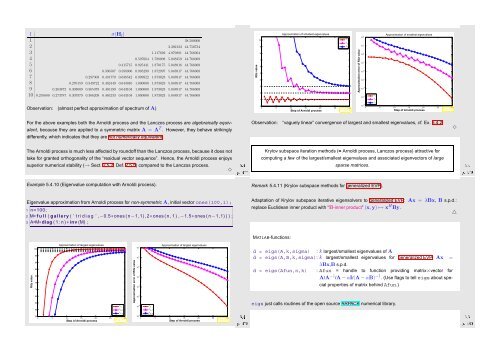
Observation: (almost perfect approximation of spectrum of A)
0
0 5 10 15 20 25 30
Step of Arnoldi process
Fig. 83
10 −6
λ 3
Fig. 84
0 5 10 15 20 25 30
For the above examples both the Arnoldi process and the Lanczos process are algebraically equivalent,
because they are applied to a symmetric matrix A = A T . However, they behave strikingly
differently, which indicates that they are not numerically equivalent.
Observation: “vaguely linear” convergence of largest and smallest eigenvalues, cf. Ex. 5.4.2.
✸
The Arnoldi process is much less affected by roundoff than the Lanczos process, because it does not
Ôº º
take for granted orthogonality of the “residual vector sequence”. Hence, the Arnoldi process enjoys
superior numerical stability (→ Sect. 2.5.2, Def. 2.5.5) compared to the Lanczos process.
✸
Krylov subspace iteration methods (= Arnoldi process, Lanczos process) attractive for
computing a few of the largest/smallest eigenvalues and associated eigenvectors of large
sparse matrices.
Ôº º
Example 5.4.10 (Eigenvalue computation with Arnoldi process).
Remark 5.4.11 (Krylov subspace methods for generalized EVP).
Eigenvalue approximation from Arnoldi process for non-symmetric A, initial vector ones(100,1);
1 n=100;
2 M= f u l l ( g a llery ( ’ t r i d i a g ’ ,−0.5∗ones ( n−1,1) ,2∗ ones ( n , 1 ) ,−1.5∗ones ( n−1,1) ) ) ;
3 A=M∗diag ( 1 : n ) ∗inv (M) ;
Adaptation of Krylov subspace iterative eigensolvers to generalized EVP: Ax = λBx, B s.p.d.:
replace Euclidean inner product with “B-inner product” (x,y) ↦→ x H By.
△
MATLAB-functions:
Ritz value
100
95
90
85
80
75
70
65
60
55
Approximation of largest eigenvalues
50
0 5 10 15 20 25 30
Step of Arnoldi process
Fig. 81
λ n
λ n−1
λ n−2
Approximation error of Ritz value
Approximation of largest eigenvalues
10 2
10 1
10 0
10 −1
10 −2
10 −3
10 −4 λ n
λ n−1
10 −5
0 5 10 15 20 25 30
Step of Arnoldi process
λ n−2
Ôº º
Fig. 82
d = eigs(A,k,sigma) : k largest/smallest eigenvalues of A
d = eigs(A,B,k,sigma): k largest/smallest eigenvalues for generalized EVP Ax =
λBx,B s.p.d.
d = eigs(Afun,n,k) : Afun = handle to function providing matrix×vector for
A/A −1 /A − αI/(A − αB) −1 . (Use flags to tell eigs about special
properties of matrix behind Afun.)
eigs just calls routines of the open source ARPACK numerical library.
Ôº¼ º