Numerical Methods Contents - SAM

Recall:
e i ˆ= i-th unit vector
Changing a single row: given x ∈ K n
{
A,Ã ∈ Kn,n a
: ã ij = ij , if i ≠ i ∗ ,
x j + a ij , if i = i ∗ ,
à = A + x · e i ∗e T j ∗ . (2.9.2)
, i ∗ ,j ∗ ∈ {1, ...,n} .
Apply Lemma 2.9.1 for k = 1:
x = ( I −
A−1 uv H )
A −1 1 + v H A −1 b .
u
Efficient implementation !
Code 2.9.4: solving a rank-1 modified LSE
1 function x = smw( L ,U, u , v , b )
2 t = L \ b ; z = U\ t ;
3 t = L \ u ; w = U\ t ;
4 alpha = 1+dot ( v ,w) ;
5 i f ( abs ( alpha ) < eps∗norm(U, 1 ) ) ,
➤
error ( ’ Nearly s i n g u l a r
m a trix ’ ) ; end ;
6 x = z − w∗dot ( v , z ) / alpha ;
△
à = A + e i ∗x T . (2.9.3)
The approach of Rem. 2.9.3 is certainly efficient, but may suffer from instability similar to Gaussian
elimination without pivoting, cf. Ex. 2.3.1.
Both matrix modifications (2.9.1) and (2.9.3) are specimens of a rank-1-modifications.
This can be avoided by using QR-factorization (→ Sect. 2.8) and corresponding update techniques.
This is the principal rationale for studying QR-factorization for the solution of linear system of equations.
✸
Ôº¾½ ¾º
Other important applications of QR-factorization will be discussed later in Chapter 6.
Ôº¾½ ¾º
A ∈ K n,n ↦→ Ã := A + uvH , u,v ∈ K n . (2.9.4)
Task:
Efficient computation of QR-factorization (→ Sect. 2.8) à = ˜Q˜R of à from (2.9.4), when
QR-factorization A = QR already known
Remark 2.9.3 (Solving LSE in the case of rank-1-modification).
general rank-1-matrix
1 With w := Q H u: A + uv H = Q(R + wv H )
➡
Asymptotic complexity O(n 2 ) (depends on how Q is stored)
✬
✩
Lemma 2.9.1 (Sherman-Morrison-Woodbury formula). For regular A ∈ K n,n , and U,V ∈
K n,k , n, k ∈ N, k ≤ n, holds
if
✫
(A + UV H ) −1 = A −1 − A −1 U(I + V H A −1 U) −1 V H A −1 ,
I + V H A −1 U regular.
Task: Solve Ãx = b, when LU-factorization A = LU already known
✪
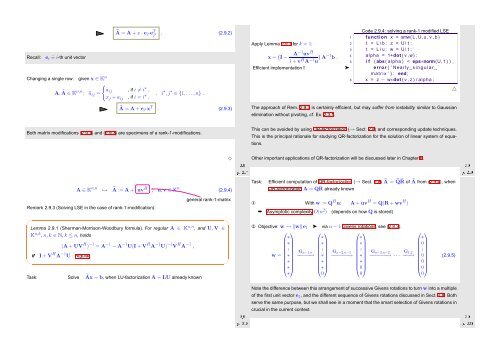
2 Objective: w → ‖w‖e 1 ➤ via n − 1 Givens rotations, see (2.8.3).
⎛ ⎞ ⎛ ⎞ ⎛ ⎞
⎛ ⎞
∗
∗
∗
∗
∗.
G
w =
∗
n−1,n
∗.
G −−−−−→
∗
n−2,n−1
∗.
G −−−−−−→
∗
n−3,n−2 G 1,2
0.
−−−−−−→ · · · −−−→
0
⎜
∗
⎟ ⎜
∗
⎟ ⎜
∗
⎟
⎜
0
⎟
⎝∗⎠
⎝∗⎠
⎝0⎠
⎝0⎠
∗ 0
0
0
(2.9.5)
Ôº¾½ ¾º
Note the difference between this arrangement of successive Givens rotations to turn w into a multiple
of the first unit vector e 1 , and the different sequence of Givens rotations discussed in Sect. 2.8. Both
serve the same purpose, but we shall see in a moment that the smart selection of Givens rotations in
crucial in the current context.
Ôº¾¾¼ ¾º