Numerical Methods Contents - SAM

More documents

Recommendations

Info

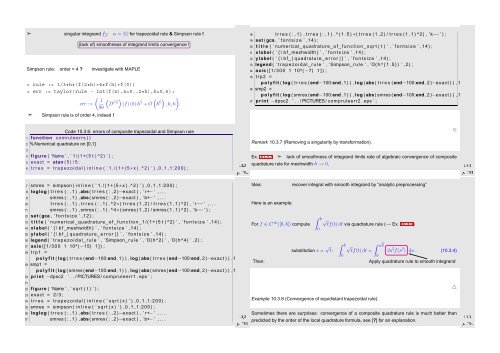
➣ singular integrand f 2 : α = 3/2 for trapezoidal rule & Simpson rule ! (lack of) smoothness of integrand limits convergence ! Simpson rule: order = 4 ? investigate with MAPLE > rule := 1/3*h*(f(2*h)+4*f(h)+f(0)) > err := taylor(rule - int(f(x),x=0..2*h),h=0,6); ( 1 ( err := D (4)) ( (f) (0)h 5 + O h 6) ) ,h, 6 90 28 t r r e s ( : , 1 ) , t r r e s ( : , 1 ) . ^ ( 1 . 5 ) ∗( t r r e s ( 1 , 2 ) / t r r e s ( 1 , 1 ) ^2) , ’ k−−’ ) ; 29 set ( gca , ’ f o n t s i z e ’ ,14) ; 30 t i t l e ( ’ numerical quadrature o f f u n c t i o n s q r t ( t ) ’ , ’ f o n t s i z e ’ ,14) ; 31 xlabel ( ’ { \ b f meshwidth } ’ , ’ f o n t s i z e ’ ,14) ; 32 ylabel ( ’ { \ b f | quadrature e r r o r | } ’ , ’ f o n t s i z e ’ ,14) ; 33 legend ( ’ t r a p e z o i d a l r u l e ’ , ’ Simpson r u l e ’ , ’O( h ^ { 1 . 5 } ) ’ ,2) ; 34 axis ( [ 1 / 3 0 0 1 10^(−7) 1 ] ) ; 35 t r p 2 = p o l y f i t ( log ( t r r e s ( end−100:end , 1 ) ) , log ( abs ( t r r e s ( end−100:end , 2 )−exact ) ) ,1) 36 smp2 = p o l y f i t ( log ( smres ( end−100:end , 1 ) ) , log ( abs ( smres ( end−100:end , 2 )−exact ) ) ,1) 37 p r i n t −dpsc2 ’ . . / PICTURES/ compruleerr2 . eps ’ ; ➣ Simpson rule is of order 4, indeed ! Code 10.3.6: errors of composite trapezoidal and Simpson rule 1 function comruleerrs ( ) 2 % <strong>Numerical</strong> quadrature on [0,1] Ôº½ ½¼º¿ 6 t r r e s = t r a p e z o i d a l ( i n l i n e ( ’ 1 . / ( 1 + ( 5∗ x ) . ^ 2 ) ’ ) ,0 ,1 ,1:200) ; 3 4 figure ( ’Name ’ , ’ 1 /(1+(5 t ) ^2) ’ ) ; 5 exact = atan ( 5 ) / 5 ; ✸ Remark 10.3.7 (Removing a singularity by transformation). Ex. 10.3.3 ➣ lack of smoothness of integrand limits rate of algebraic convergence of composite quadrature rule for meshwidth h → 0. Ôº¿ ½¼º¿ 7 smres = simpson ( i n l i n e ( ’ 1 . / ( 1 + ( 5∗ x ) . ^ 2 ) ’ ) ,0 ,1 ,1:200) ; 8 loglog ( t r r e s ( : , 1 ) , abs ( t r r e s ( : , 2 )−exact ) , ’ r+− ’ , . . . 9 smres ( : , 1 ) , abs ( smres ( : , 2 )−exact ) , ’ b+− ’ , . . . 10 t r r e s ( : , 1 ) , t r r e s ( : , 1 ) . ^ 2∗( t r r e s ( 1 , 2 ) / t r r e s ( 1 , 1 ) ^2) , ’ r−−’ , . . . 11 smres ( : , 1 ) , smres ( : , 1 ) . ^ 4∗( smres ( 1 , 2 ) / smres ( 1 , 1 ) ^2) , ’ b−−’ ) ; 12 set ( gca , ’ f o n t s i z e ’ ,12) ; 13 t i t l e ( ’ numerical quadrature o f f u n c t i o n 1 /(1+(5 t ) ^2) ’ , ’ f o n t s i z e ’ ,14) ; 14 xlabel ( ’ { \ b f meshwidth } ’ , ’ f o n t s i z e ’ ,14) ; 15 ylabel ( ’ { \ b f | quadrature e r r o r | } ’ , ’ f o n t s i z e ’ ,14) ; 16 legend ( ’ t r a p e z o i d a l r u l e ’ , ’ Simpson r u l e ’ , ’O( h ^2) ’ , ’O( h ^4) ’ ,2) ; 17 axis ( [ 1 / 3 0 0 1 10^(−15) 1 ] ) ; 18 t r p 1 = p o l y f i t ( log ( t r r e s ( end−100:end , 1 ) ) , log ( abs ( t r r e s ( end−100:end , 2 )−exact ) ) ,1) 19 smp1 = p o l y f i t ( log ( smres ( end−100:end , 1 ) ) , log ( abs ( smres ( end−100:end , 2 )−exact ) ) ,1) 20 p r i n t −dpsc2 ’ . . / PICTURES/ compruleerr1 . eps ’ ; 21 22 figure ( ’Name ’ , ’ s q r t ( t ) ’ ) ; 23 exact = 2 / 3 ; 24 t r r e s = t r a p e z o i d a l ( i n l i n e ( ’ s q r t ( x ) ’ ) ,0 ,1 ,1:200) ; Ôº¾ ½¼º¿ 25 smres = simpson ( i n l i n e ( ’ s q r t ( x ) ’ ) ,0 ,1 ,1:200) ; 26 loglog ( t r r e s ( : , 1 ) , abs ( t r r e s ( : , 2 )−exact ) , ’ r+− ’ , . . . 27 smres ( : , 1 ) , abs ( smres ( : , 2 )−exact ) , ’ b+− ’ , . . . Idea: Here is an example: For f ∈ C ∞ ([0,b]) compute Then: recover integral with smooth integrand by “analytic preprocessing” substitution s = √ t: ∫ b √ tf(t) dt via quadrature rule (→ Ex. 10.3.3) Example 10.3.8 (Convergence of equidistant trapezoidal rule). 0 ∫ b √ ∫ √ b tf(t) dt = 2s 2 f(s 2 ) ds . (10.3.4) 0 0 Apply quadrature rule to smooth integrand Sometimes there are surprises: convergence of a composite quadrature rule is much better than predicted by the order of the local quadrature formula, see [?] for an explanation. △ Ôº ½¼º¿
Equidistant trapezoidal rule (order 2), see (10.3.2) ∫ b a ( m−1 ∑ ) f(t) dt ≈ T m (f) := h 12 f(a) + f(kh) + 2 1f(b) , h := b − a m . (10.3.5) k=1 Code 10.3.9: equidistant trapezoidal quadrature formula 1 function res = t r a p e z o i d a l ( f n c t , a , b ,N) 2 % <strong>Numerical</strong> quadrature based on trapezoidal rule 3 % fnct handle to y = f(x) 4 % a,b bounds of integration interval 5 % N+1 = number of equidistant integration points (can be a vector) 6 res = [ ] ; 7 for n = N 8 h = ( b−a ) / n ; x = ( a : h : b ) ; w = [ 0 . 5 ones ( 1 , n−1) 0 . 5 ] ; 9 res = [ res ; h , h∗dot (w, feval ( f n c t , x ) ) ] ; 10 end 1-periodic smooth (analytic) integrand f(t) = 1 √ 1 − a sin(2πt − 1) , 0 < a < 1 . Ôº ½¼º¿ 2 3 clear a ; 4 global a ; 5 l = 0 ; r = 0 . 5 ; % integration interval 6 N = 50; 7 a = 0 . 5 ; res05 = t r a p e z o i d a l ( @issin , l , r , 1 :N) ; 8 ex05 = t r a p e z o i d a l ( @issin , l , r ,500) ; ex05 = ex05 ( 1 , 2 ) ; 9 a = 0 . 9 ; res09 = t r a p e z o i d a l ( @issin , l , r , 1 :N) ; 10 ex09 = t r a p e z o i d a l ( @issin , l , r ,500) ; ex09 = ex09 ( 1 , 2 ) ; 11 a = 0 . 9 5 ; res95 = t r a p e z o i d a l ( @issin , l , r , 1 :N) ; 12 ex95 = t r a p e z o i d a l ( @issin , l , r ,500) ; ex95 = ex95 ( 1 , 2 ) ; 13 a = 0 . 9 9 ; res99 = t r a p e z o i d a l ( @issin , l , r , 1 :N) ; 14 ex99 = t r a p e z o i d a l ( @issin , l , r ,500) ; ex99 = ex99 ( 1 , 2 ) ; 15 figure ( ’name ’ , ’ t r a p e z o i d a l r u l e f o r non−p e r i o d i c f u n c t i o n ’ ) ; 16 loglog ( 1 . / res05 ( : , 1 ) ,abs ( res05 ( : , 2 )−ex05 ) , ’ r+− ’ , . . . 17 1 . / res09 ( : , 1 ) , abs ( res09 ( : , 2 )−ex09 ) , ’ b+− ’ , . . . 18 1 . / res95 ( : , 1 ) , abs ( res95 ( : , 2 )−ex95 ) , ’ c+− ’ , . . . 19 1 . / res99 ( : , 1 ) , abs ( res99 ( : , 2 )−ex99 ) , ’m+− ’ ) ; 20 set ( gca , ’ f o n t s i z e ’ ,12) ; 21 legend ( ’ a=0.5 ’ , ’ a=0.9 ’ , ’ a=0.95 ’ , ’ a=0.99 ’ ,3) ; 22 xlabel ( ’ { \ b f no . o f . quadrature nodes } ’ , ’ f o n t s i z e ’ ,14) ; 23 ylabel ( ’ { \ b f | quadrature e r r o r | } ’ , ’ f o n t s i z e ’ ,14) ; Ôº ½¼º¿ 24 t i t l e ( ’ { \ b f Trapezoidal r u l e quadrature f o r non−p e r i o d i c (“exact value of integral”: use T 500 ) |quadrature error| Trapezoidal rule quadrature for 1./sqrt(1−a*sin(2*pi*x+1)) 10 0 10 −2 10 −4 10 −6 10 −8 10 −10 10 −12 a=0.5 a=0.9 a=0.95 a=0.99 10 −14 0 2 4 6 8 10 12 14 16 18 20 no. of. quadrature nodes Fig. 112 quadrature error for T n (f) on [0, 1] exponential convergence !! |quadrature error| Trapezoidal rule quadrature for non−periodic function 10 −1 10 −2 10 −3 10 −4 a=0.5 a=0.9 a=0.95 a=0.99 10 −5 10 0 10 1 10 2 no. of. quadrature nodes Fig. 113 10 0 quadrature error for T n (f) on [0, 1 2 ] Ôº ½¼º¿ Ôº ½¼º¿ 1 function t r a p e r r ( ) 46 legend ( ’ a=0.5 ’ , ’ a=0.9 ’ , ’ a=0.95 ’ , ’ a=0.99 ’ ,3) ; merely algebraic convergence Code 10.3.10: tracking error of equidistant trapezoidal quadrature formula 25 f u n c t i o n } ’ , ’ f o n t s i z e ’ ,12) ; 26 p r i n t −depsc2 ’ . . / PICTURES/ t r a p e r r 2 . eps ’ ; 27 28 clear a ; 29 global a ; 30 l = 0 ; r = 1 ; % integration interval 31 N = 20; 32 a = 0 . 5 ; res05 = t r a p e z o i d a l ( @issin , l , r , 1 :N) ; 33 ex05 = t r a p e z o i d a l ( @issin , l , r ,500) ; ex05 = ex05 ( 1 , 2 ) ; 34 a = 0 . 9 ; res09 = t r a p e z o i d a l ( @issin , l , r , 1 :N) ; 35 ex09 = t r a p e z o i d a l ( @issin , l , r ,500) ; ex09 = ex09 ( 1 , 2 ) ; 36 a = 0 . 9 5 ; res95 = t r a p e z o i d a l ( @issin , l , r , 1 :N) ; 37 ex95 = t r a p e z o i d a l ( @issin , l , r ,500) ; ex95 = ex95 ( 1 , 2 ) ; 38 a = 0 . 9 9 ; res99 = t r a p e z o i d a l ( @issin , l , r , 1 :N) ; 39 ex99 = t r a p e z o i d a l ( @issin , l , r ,500) ; ex99 = ex99 ( 1 , 2 ) ; 40 figure ( ’name ’ , ’ t r a p e z o i d a l r u l e f o r p e r i o d i c f u n c t i o n ’ ) ; 41 semilogy ( 1 . / res05 ( : , 1 ) , abs ( res05 ( : , 2 )−ex05 ) , ’ r+− ’ , . . . 42 1 . / res09 ( : , 1 ) , abs ( res09 ( : , 2 )−ex09 ) , ’ b+− ’ , . . . 43 1 . / res95 ( : , 1 ) , abs ( res95 ( : , 2 )−ex95 ) , ’ c+− ’ , . . . 44 1 . / res99 ( : , 1 ) , abs ( res99 ( : , 2 )−ex99 ) , ’m+− ’ ) ; 45 set ( gca , ’ f o n t s i z e ’ ,12) ;
Page 1 and 2:
2 Direct Methods for Linear Systems
Page 3 and 4:
III Integration of Ordinary Differe
Page 5 and 6:
Extra questions for course evaluati
Page 7 and 8:
1.1.2 Matrices Matrices = two-dimen
Page 9 and 10:
Remark 1.2.1 (Row-wise & column-wis
Page 11 and 12:
1.3 Complexity/computational effort
Page 13 and 14:
Syntax of BLAS calls: The functions
Page 15 and 16:
4 { 5 a ssert ( this−>n==B. n &&
Page 17 and 18:
34 long r t 0 ; 35 bool bStarted ;
Page 19 and 20:
Obviously, left multiplication with
Page 21 and 22:
❶: elimination step, ❷: backsub
Page 23 and 24:
A direct way to LU-decomposition:
Page 25 and 26:
Solution of LŨx = b: x ( ) 2ǫ = 1
Page 27 and 28:
numerically equivalent ˆ= same res
Page 29 and 30:
Code 2.4.8: Finding outeps in MATLA
Page 31 and 32:
Terminology: Def. 2.5.5 introduces
Page 33 and 34:
Example 2.5.5 (Instability of multi
Page 35 and 36:
Note: sensitivity gauge depends on
Page 37 and 38:
6 for i =1:20 7 n = 2^ i ; m = n /
Page 39 and 40:
0 20 40 60 80 100 120 140 160 180 2
Page 41 and 42:
Use sparse matrix format: 10 1 10 2
Page 43 and 44:
Envelope-aware LU-factorization: 0
Page 45 and 46:
0 20 40 60 80 100 0 20 0 20 0 20 De
Page 47 and 48:
Evident: symmetry of Ã − bbT a 1
Page 49 and 50:
9 ylabel ( ’ { \ b f c o n d i t
Page 51 and 52:
Mapping a ∈ K n to a multiple of
Page 53 and 54:
Then store G ij (a,b) as triple (i,
Page 55 and 56:
Recall: e i ˆ= i-th unit vector Ch
Page 57 and 58:
Computation of Choleskyfactorizatio
Page 59 and 60:
1 ∃ (partial) cyclic row permutat
Page 61 and 62:
Definition 3.1.3 (Local and global
Page 63 and 64:
Example 3.1.6 (quadratic convergenc
Page 65 and 66:
k |x (k) − π| L 1−L |x (k) −
Page 67 and 68:
(x (k) ) k∈N0 Cauchy sequence ➤
Page 69 and 70:
Termination criterion for contracti
Page 71 and 72:
Given x (k) ∈ I, next iterate :=
Page 73 and 74:
secant method ( MATLAB implementati
Page 75 and 76:
Assuming p = 1: p > 1: ∥ C ∥e (
Page 77 and 78:
This is a simple computation: DG(x)
Page 79 and 80:
k x (k) ǫ k := ‖x ∗ − x (k)
Page 81 and 82:
Code 3.4.14: Damped Newton method (
Page 83 and 84:
MATLAB-CODE: Broyden method (3.4.11
Page 85 and 86:
Algorithm 4.1.3 (Steepest descent).
Page 87 and 88:
Example 4.1.8 (Convergence of gradi
Page 89 and 90:
4.2.1 Krylov spaces Definition 4.2.
Page 91 and 92:
Remark 4.2.3 (A posteriori terminat
Page 93 and 94:
10 figure ; view ([ −45 ,28]) ; m
Page 95 and 96:
Idea: Solve Ax = b approximately in
Page 97 and 98:
eplaced with κ(A) ! 4.4.2 Iteratio
Page 99 and 100:
For circuit of Fig. 55 at angular f
Page 101 and 102:
(Linear) generalized eigenvalue pro
Page 103 and 104:
10 0 10 1 matrix size n d = eig(A)
Page 105 and 106:
0 50 100 150 200 250 300 350 400 45
Page 107 and 108:
1 2 3 k ρ (k) EV ρ (k) EW ρ (k)
Page 109 and 110:
✬ ✩ ✬ ✩ Lemma 5.3.4 (Ncut a
Page 111 and 112:
In other words, roundoff errors may
Page 113 and 114:
Theory: linear convergence of (5.3.
Page 115 and 116:
error in eigenvalue 10 0 10 −2 10
Page 117 and 118:
✬ Residuals r 0 ,...,r m−1 gene
Page 119 and 120:
Algebraic view of the Arnoldi proce
Page 121 and 122:
5.5 Singular Value Decomposition Re
Page 123 and 124:
Illustration: columns = ONB of Im(A
Page 125 and 126:
✬ Theorem 5.5.7 (best low rank ap
Page 127 and 128:
Reassuring: Remark 6.0.4 (Pseudoinv
Page 129 and 130:
Consider the linear least squares p
Page 131 and 132:
Goal: Euclidean distance of y ∈ R
Page 133 and 134:
6.5 Non-linear Least Squares If (6.
Page 135 and 136:
0 2 4 6 8 10 12 14 16 value of ∥
Page 137 and 138:
Definition 7.1.1 (Discrete convolut
Page 139 and 140:
Expand a 0 ,...,a n−1 and b 0 , .
Page 141 and 142:
(7.2.2) is a simple consequence of
Page 143 and 144:
Dominant coefficients of a signal a
Page 145 and 146: 11 c = f f t ( y ) ; 12 13 figure (
Page 147 and 148: Two-dimensional trigonometric basis
Page 149 and 150: 8 end 9 t1 = min ( t1 , toc ) ; 10
Page 151 and 152: Step II: for k =: rq + s, 0 ≤ r <
Page 153 and 154: MATLAB-CODE Sine transform function
Page 155 and 156: △ Example 7.5.2 (Linear regressio
Page 157 and 158: [23, Ch. IX] presents the topic fro
Page 159 and 160: Code 8.1.3: Horner scheme, polynomi
Page 161 and 162: 1.2 equality in (8.2.10) for y := (
Page 163 and 164: ecursive definition: p i (t) ≡ y
Page 165 and 166: a 1 = y 1 − a 0 t 1 − t 0 = y 1
Page 167 and 168: Observations: Strong oscillations o
Page 169 and 170: −1 −0.8 −0.6 −0.4 −0.2 0
Page 171 and 172: 8.5.3 Chebychev interpolation: comp
Page 173 and 174: 9.1 Shape preserving interpolation
Page 175 and 176: 9.2.2 Piecewise polynomial interpol
Page 177 and 178: Interpolation of the function: f(x)
Page 179 and 180: 2 % Plot convergence of approximati
Page 181 and 182: 9.4 Splines Definition 9.4.1 (Splin
Page 183 and 184: ➤ Linear system of equations with
Page 185 and 186: y i+1 t i−1 t i t i+1 y i−1 y i
Page 187 and 188: 35 h= d i f f ( t ) ; 36 d e l t a
Page 189 and 190: 1 0.9 Function f 1 0.9 Function f
Page 191 and 192: f 10 Numerical Quadrature Numerical
Page 193 and 194: f • n = 1: Trapezoidal rule • n
Page 195: For fixed local n-point quadrature
Page 199 and 200: Heuristics: A quadrature formula ha
Page 201 and 202: 20 Zeros of Legendre polynomials in
Page 203 and 204: |quadrature error| 10 0 Numerical q
Page 205 and 206: f f • line 9: estimate for global
Page 207 and 208: Model: autonomous Lotka-Volterra OD
Page 209 and 210: Example 11.1.6 (Transient circuit s
Page 211 and 212: y y 1 y(t) y 0 t t 0 t 1 Fig. 133 e
Page 213 and 214: for discrete evolution defined on I
Page 215 and 216: ⇒ if y ∈ C 2 ([0, T]), then y(t
Page 217 and 218: The implementation of an s-stage ex
Page 219 and 220: Example 11.5.2 (Blow-up). ✸ toler
Page 221 and 222: However, it would be foolish not to
Page 223 and 224: 0 0.2 0.4 0.6 0.8 1 1.2 1.4 1.6 1.8
Page 225 and 226: 4 3 2 abstol = 0.000010, reltol = 0
Page 227 and 228: ✸ ✸ Motivated by the considerat
Page 229 and 230: 0 1 2 3 4 5 6 u(t),v(t) 0.01 0.008
Page 231 and 232: MATLAB-CODE : Explicit integration
Page 233 and 234: Shorthand notation for Runge-Kutta
Page 235 and 236: 13 Structure Preservation 13.1 Diss
Page 237 and 238: [18] G. GOLUB AND C. VAN LOAN, Matr
Page 239 and 240: linear in Gauss-Newton method, 538
Page 241 and 242: Chebychev nodes, 678 double, 634 fo
Page 243 and 244: x∗ n y ˆ= discrete periodic conv
Page 245 and 246: Gaussian elimination with pivoting
show all

Numerical Methods Contents - SAM

You also want an ePaper? Increase the reach of your titles

Delete template?

Save as template?