Numerical Methods Contents - SAM

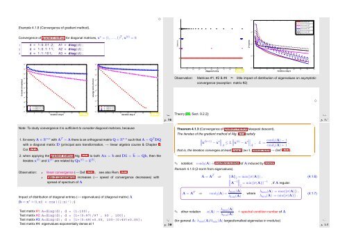
Example 4.1.8 (Convergence of gradient method).
✸
#4
10 2
error norm, #1
norm of residual, #1
error norm, #2
norm of residual, #2
error norm, #3
norm of residual, #3
error norm, #4
norm of residual, #4
Convergence of gradient method for diagonal matrices, x ∗ = (1,...,1) T , x (0) = 0:
#3
1 d = 1 : 0 . 0 1 : 2 ; A1 = diag ( d ) ;
2 d = 1 : 0 . 1 : 1 1 ; A2 = diag ( d ) ;
3 d = 1 : 1 : 1 0 1 ; A3 = diag ( d ) ;
matrix no.
#2
2−norms
10 1
10 0
#1
10 2
10 0
0 10 20 30 40 50 60 70 80 90 100
diagonal entry
Fig. 48
10 3 iteration step k
10 −1
0 5 10 15 20 25 30 35 40 45
2−norm of residual
step
10 0
10 −2
10 −4
10 −6
10 −8
10 −10
10 −12
10 −14 A = diag(1:0.01:2)
A = diag(1:0.1:11)
A = diag(1:1:101)
10 −16
0 5 10 15 20
iteration
25
k
30 35 40
Fig. 46
10 4
energy norm of error
step
10 −2
10 −4
10 −6
10 −8
10 −10
10 −12
10 −14 A = diag(1:0.01:2)
A = diag(1:0.1:11)
A = diag(1:1:101)
10 −16
0 5 10 15 20
iteration
25
k
30 35 40
Fig. 47
10 2
Ôº¿ º½
Observation: Matrices #1, #2 & #4 ➣ little impact of distribution of eigenvalues on asymptotic
convergence (exception: matrix #2)
✸
Theory [20, Sect. 9.2.2]:
Ôº¿ º½
Note: To study convergence it is sufficient to consider diagonal matrices, because
1. for every A ∈ R n,n with A T = A there is an orthogonal matrix Q ∈ R n.n such that A = Q T DQ
with a diagonal matrix D (principal axis transformation, → linear algebra course & Chapter 5,
Cor. 5.1.7),
2. when applying the gradient method Alg. 4.1.4 to both Ax = b and D˜x = ˜b := Qb, then the
iterates x (k) and ˜x (k) are related by Qx (k) = ˜x (k) .
Observation: linear convergence (→ Def. 3.1.4), see also Rem. 3.1.3
rate of convergence increases (↔ speed of convergence decreases) with
spread of spectrum of A
✬
Theorem 4.1.3 (Convergence of gradient method/steepest descent).
The iterates of the gradient method of Alg. 4.1.4 satisfy
∥
∥x (k+1) − x ∗∥ ∥ ∥ ∥A ≤ L∥x (k) − x ∗∥ ∥ ∥A , L := cond 2(A) − 1
cond 2 (A) + 1 ,
that is, the iteration converges at least linearly (w.r.t. energy norm → Def. 4.1.1).
✫
✎ notation: cond 2 (A) ˆ= condition number of A induced by 2-norm
Remark 4.1.9 (2-norm from eigenvalues).
A = A T ⇒ ‖A‖ 2 = max(|σ(A)|) ,
∥
∥A −1∥ ∥ ∥2 = min(|σ(A)|) −1
, if A regular.
(4.1.6)
✩
✪
Impact of distribution of diagonal entries (↔ eigenvalues) of (diagonal matrix) A
(b = x ∗ = 0, x0 = cos((1:n)’);)
A = A T ⇒ cond 2 (A) = λ max(A)
λ min (A) , where λ max (A) := max(|σ(A)|) ,
λ min (A) := min(|σ(A)|) .
(4.1.7)
Test matrix #1: A=diag(d); d = (1:100);
Test matrix #2: A=diag(d); d = [1+(0:97)/97 , 50 , 100];
Test matrix #3: A=diag(d); d = [1+(0:49)*0.05, 100-(0:49)*0.05];
Test matrix #4: eigenvalues exponentially dense at 1
Ôº¿ º½
✎ other notation κ(A) := λ max(A)
λ min (A)
ˆ= spectral condition number of A
(for general A: λ max (A)/λ min (A) largest/smallest eigenvalue in modulus)
Ôº¿ º½