Numerical Methods Contents - SAM

ecursive definition:
p i (t) ≡ y i , i = 0,...,n ,
p i0 ,...,i m
(t) = (t − t i 0
)p i1 ,...,i m
(t) − (t − t im )p i0 ,...,i m−1
(t)
t im − t i0
.
Aitken-Neville algorithm:
n = 0 1 2 3
t 0 y 0 =: p 0 (x) → ր
p 01 (x) → ր
p 012 (x) → ր
p 0123 (x)
t 1 y 1 =: p 1 (x) → ր
p 12 (x) → ր
p 123 (x)
t 2 y 2 =: p 2 (x) → ր
p 23 (x)
t 3 y 3 =: p 3 (x)
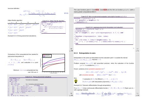
Example 8.3.3 (Timing polynomial evaluations).
Comparison of the computational time needed for
polynomial interpolation of
{t i = i} i=1,...,n , {y i = √ i} i=1,...,n ,
n = 3, ...,200, and evaluation in a point
x ∈ [0,n].
Minimum tic-toc-computational time
Code 8.3.2: Aitken-Neville algorithm
1 function v = ANipoleval ( t , y , x )
2 for i =1: length ( y )
3 for k= i −1:−1:1
4 y ( k ) = y ( k +1) +( y ( k +1)−y ( k ) ) ∗ . . .
5 ( x−t ( i ) ) / ( t ( i )−t ( k ) ) ;
6 end
7 end
8 v = y ( 1 ) ;
Computational time [s]
10 0 Aitken−Neville scheme
MATLAB polyfit
Barycentric formula
10 −1
Legendre polynomials
10 −2
10 −3
10 −4
Polynomial degree
10
0 20 40 60 80 100 120 140 160 180 200
over 100 runs ➙ −5
Code 8.3.4: Timing polynomial evaluations
(8.3.2)
Ôº º¿
1 time=zeros ( 1 , 4 ) ;
2 f =@( x ) sqrt ( x ) ; % function to interpolate:
3 for k=1:100
4 res = [ ] ;
5 for n=3:1:200 % n = increasing polynomial degree
6 t = ( 1 : n ) ; y = f ( t ) ; x=n∗rand ;
14 else , f i n r e s = min ( f i n r e s , res ) ; end
7 t i c ; v1 = ANipoleval ( t , y , x ) ; time ( 1 ) = toc ;
8 t i c ; v2 = i p o l e v a l ( t , y , x ) ; time ( 2 ) = toc ;
9 t i c ; v3 = i n t p o l y v a l ( t , y , x ) ; time ( 3 ) = toc ;
10 t i c ; v4 = i n t p o l y v a l _ l a g ( t , y , x ) ; time ( 4 ) = toc ;
11 res = [ res ; n , time ] ;
12 end
13 i f ( k == 1) , f i n r e s = res ; Ôº¼ º¿
This uses functions given in Code 8.3.0, Code 8.3.1 and the MATLAB function polyfit (with a
clearly greater computational effort !)
Code 8.3.5: MATLAB polynomial evaluation using built-in function polyfit
1 function v= i p o l e v a l ( t , y , x )
2 p = p o l y f i t ( t , y , length ( y )−1) ;
3 v=polyval ( p , x ) ;
Code 8.3.6: Lagrange polynomial interpolation and evaluation
1 function p = i n t p o l y v a l _ l a g ( t , y , x )
2 p=zeros ( size ( x ) ) ;
3 for k =1: length ( t ) ; p=p + y ( k ) ∗ lagrangepoly ( x , k−1, t ) ; end
4
5 function L=lagrangepoly ( x , index , nodes )
6 L=1;
7 for j = [ 0 : index −1, index +1: length ( nodes ) −1];
8 L = L .∗ ( x−nodes ( j +1) ) . / ( nodes ( index +1)−nodes ( j +1) ) ;
9 end
8.3.3 Extrapolation to zero
Extrapolation is the same as interpolation but the evaluation point t is outside the interval
[inf j=0,...,n t j , sup j=0,...,n t j ]. Assume t = 0.
Problem: compute lim t→0 f(t) with prescribed precision, when the evaluation of the function
y=f(t) is unstable for |t| ≪ 1.
Known: existence of an asymptotic expansion in h 2
Idea:
f(h) = f(0) + A 1 h 2 + A 2 h 4 + · · · + A n h 2n + R(h) , A k ∈ K ,
with remainder estimate |R(h)| = O(h 2n+2 ) for h → 0 .
➀ evaluation of f(t i ) for different t i , i = 0,...,n, |t i | > 0.
➁ f(0) ≈ p(0) with interpolation polynomial p ∈ P n , p(t i ) = f(t i ).
Example 8.3.7 (Numeric differentiation through extrapolation).
For a 2(n + 1)-times continuously differentiable function f : D ⊂ R ↦→ R, x ∈ D (Taylor sum in x
with Lagrange residual)
n∑
T(h) :=
f(x + h) − f(x − h)
2h
∼ f ′ 1 d 2k f
(x) +
(2k)! dx
k=1
2k(x)h2k +
1
Ôº½ º¿ ✸
Ôº¾ º¿
(2n + 2)! f(2n+2) (ξ(x)) .