Numerical Methods Contents - SAM

ootstrapping = use the same idea in a simpler version to get y(t 0 + c i h), noting that these values
can be replaced by other approximations obtained by methods already constructed (this approach
will be elucidated in the next example).
1
0.9
0.8
0.7
y(t)
Explicit Euler
Explicit trapezoidal rule
Explicit midpoint rule
10 −1
s=1, Explicit Euler
s=2, Explicit trapezoidal rule
s=2, Explicit midpoint rule
O(h 2 )
What error can we afford in the approximation of y(t 0 +c i h) (under the assumption that f is Lipschitz
continuous)?
y
0.6
0.5
0.4
0.3
error |y h
(1)−y(1)|
10 −2
10 −3
0.2
10 −4
Goal: one-step error y(t 1 ) − y 1 = O(h p+1 )
0.1
0
0 0.2 0.4 0.6 0.8 1
t
Fig. 142
10 0 stepsize h
10 −2 10 −1
Fig. 143
This goal can already be achieved, if only
y h (j/10), j = 1,...,10 for explicit RK-methods
Errors at final time y h (1) − y(1)
y(t 0 + c i h) is approximated up to an error O(h p ),
because in (11.4.1) a factor of size h multiplies f(t 0 + c i ,y(t 0 + c i h)).
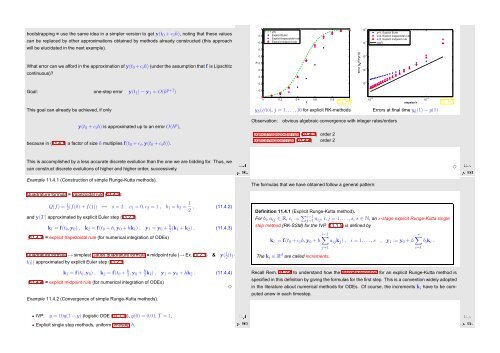
Observation:
obvious algebraic convergence with integer rates/orders
explicit trapezoidal rule (11.4.3) order 2
explicit midpoint rule (11.4.4) order 2
This is accomplished by a less accurate discrete evolution than the one we are bidding for. Thus, we
can construct discrete evolutions of higher and higher order, successively.
Ôº½ ½½º
Ôº¿ ½½º ✸
Example 11.4.1 (Construction of simple Runge-Kutta methods).
The formulas that we have obtained follow a general pattern:
Quadrature formula = trapezoidal rule (11.4.2):
Q(f) = 1 2 (f(0) + f(1)) ↔ s = 2: c 1 = 0,c 2 = 1 , b 1 = b 2 = 1 2 , (11.4.2)
and y(T) approximated by explicit Euler step (11.2.1)
k 1 = f(t 0 ,y 0 ) , k 2 = f(t 0 + h,y 0 + hk 1 ) , y 1 = y 0 + h 2 (k 1 + k 2 ) . (11.4.3)
(11.4.3) = explicit trapezoidal rule (for numerical integration of ODEs)
Quadrature formula → simplest Gauss quadrature formula = midpoint rule (→ Ex. 10.2.1) & y( 1 2 (t 1+
t 0 )) approximated by explicit Euler step (11.2.1)
Definition 11.4.1 (Explicit Runge-Kutta method).
For b i ,a ij ∈ R, c i := ∑ i−1
j=1 a ij, i,j = 1, ...,s, s ∈ N, an s-stage explicit Runge-Kutta single
step method (RK-SSM) for the IVP (11.1.5) is defined by
∑i−1
s∑
k i := f(t 0 + c i h,y 0 + h a ij k j ) , i = 1, ...,s , y 1 := y 0 + h b i k i .
j=1
The k i ∈ R d are called increments.
i=1
k 1 = f(t 0 ,y 0 ) , k 2 = f(t 0 + h 2 ,y 0 + h 2 k 1) , y 1 = y 0 + hk 2 . (11.4.4)
(11.4.4) = explicit midpoint rule (for numerical integration of ODEs)
✸
Example 11.4.2 (Convergence of simple Runge-Kutta methods).
IVP: ẏ = 10y(1 − y) (logistic ODE (11.1.1)), y(0) = 0.01, T = 1,
Explicit single step methods, uniform timestep h.
Ôº¾ ½½º
Recall Rem. 11.2.4 to understand how the discrete evolution for an explicit Runge-Kutta method is
specified in this definition by giving the formulas for the first step. This is a convention widely adopted
in the literature about numerical methods for ODEs. Of course, the increments k i have to be computed
anew in each timestep.
Ôº ½½º