Numerical Methods Contents - SAM

0
0
: diagonal
2
2
4
4
m
: super-diagonals
6
6
: sub-diagonals
8
8
n
✁ m(A) = 2, m(A) = 1
10
12
14
10
12
14
for banded matrix A ∈ K m,n :
nnz(A) ≤ min{m, n}m(A)
16
18
16
18
MATLAB function for creating banded matrices:
dense matrix : X=diag(v);
sparse matrix : X=spdiags(B,d,m,n); (sparse storage !)
tridiagonal matrix : X=gallery(’tridiag’,c,d,e); (sparse storage !)
We now examine a generalization of the concept of a banded matrix that is particularly useful in the
context of Gaussian elimination:
Ôº½ ¾º
20
0 2 4 6 8 10 12 14 16 18 20
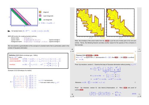
nz = 138 Fig. 17
20
0 2 4 6 8 10 12 14 16 18 20
nz = 121 Fig. 18
Note: the envelope of the arrow matrix from Ex. 2.6.13 is just the set of index pairs of its non-zero
entries. Hence, the following theorem provides another reason for the sparsity of the LU-factors in
that example.
Ôº½ ¾º
✸
✬
✩
Definition 2.6.5 (Matrix envelope (ger.: Hülle)).
For A ∈ K n,n define
row bandwidth
column bandwidth
envelope env(A) :=
Example 2.6.23 (Envelope of a matrix).
⎛
⎞
∗ 0 ∗ 0 0 0 0
0 ∗ 0 0 ∗ 0 0
∗ 0 ∗ 0 0 0 ∗
A =
0 0 0 ∗ ∗ 0 ∗
⎜
0 ∗ 0 ∗ ∗ ∗ 0
⎟
⎝ 0 0 0 0 ∗ ∗ 0 ⎠
0 0 ∗ ∗ 0 0 ∗
m R i (A) := max{0, i − j : a ij ≠ 0, 1 ≤ j ≤ n},i ∈ {1, ...,n}
m C j (A) := max{0,j − i : a ij ≠ 0, 1 ≤ i ≤ n},j ∈ {1, ...,n}
{
}
(i,j) ∈ {1,...,n} 2 i − m R : i (A) ≤ j ≤ i ,
j − m C j (A) ≤ i ≤ j
m R 1 (A) = 0
m R 2 (A) = 0
m R 3 (A) = 2
m R 4 (A) = 0
m R 5 (A) = 3
m R 6 (A) = 1
m R 7 (A) = 4
env(A) = red elements
∗ ˆ= non-zero matrix entry a ij ≠ 0
Ôº½ ¾º
Theorem 2.6.6 (Envelope and fill-in).
If A ∈ K n,n is regular with LU-decomposition A = LU, then fill-in (→ Def. 2.6.3) is confined
to
✫
env(A).
Proof. (by induction, version I) Examine first step of Gaussian elimination without pivoting, a 11 ≠ 0
(
a11 b
A =
T ) ( )( 1 0 a11 b T )
=
c à −a c I
} {{ 11 0 Ã −
}
cbT
a
} {{ 11
}
L (1) { U (1)
ci−1 = 0 , if i > j ,
If (i, j) ∉ env(A) ⇒
b j−1 = 0 , if i < j .
Moreover, env(Ã − cbT
a 11
) = env(A(2 : n, 2 : n))
⇒ env(L (1) ) ⊂ env(A), env(U (1) ) ⊂ env(A) .
Proof. (by induction, version II) Use block-LU-factorization, cf. Rem. 2.2.8 and proof of
Lemma 2.2.3:
( ) ( )(
à b ˜L 0 Ũ u
Ôº½ ¾º
)
c T =
α l T ⇒ ŨT l = c ,
(2.6.3)
1 0 ξ ˜Lu = b .
✪
✷