Numerical Methods Contents - SAM

34 long r t 0 ;
35 bool bStarted ;
36 } ;
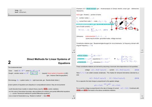
Example 2.0.1 (Nodal analysis (ger.: Knotenanalyse) of (linear) electric circuit (ger.: elektrisches
Netzwerk)).
Node (ger.: Knoten) ˆ= junction of wires
☞ number nodes 1, ...,n
➀
C 1 ➁ R 1 ➂
I kj : current from node k → node j, I kj = −I jk
U ~ L
R
Kirchhoff current law (KCL, ger.: Kirchhoffsche Knotenregel): 5
R 2
C 2
sum of node currents = 0:
R4 R 3
∑ n
∀k ∈ {1, . ..,n}:
j=1 I kj = 0 . (2.0.1)
➃ ➄ ➅
Unknowns:
nodal potentials U k , k = 1,...,n.
(some may be known: grounded nodes, voltage sources)
Ôº ½º
Constitutive relations (ger.: Bauelementgleichungen) for circuit elements: (in frequency domain with
angular frequency ω > 0):
Ôº ¾º¼
2
Direct Methods for Linear Systems of
Equations
The fundamental task:
Given : matrix A ∈ K n,n , vector b ∈ K n , n ∈ K
Sought : solution vector x ∈ K n : Ax = b ← (square) linear system of equations (LSE)
: (ger.: lineares Gleichungssystem)
(Terminology: A ˆ= system matrix, b ˆ= right hand side, ger.: Rechte-Seite-Vektor )
Linear systems of equations are ubiquitous in computational science: they are encountered
• Ohmic resistor: I = U , [R] = 1VA−1
⎧
R ⎪⎨ R −1 (U k − U j ) ,
• capacitor: I = iωCU, capacitance [C] = 1AsV −1 ➤ I kj = iωC(U k − U j ) ,
• coil/inductor : I = U
⎪⎩
iωL , inductance [L] = 1VsA−1 −iω −1 L −1 (U k − U j ) .
These constitutive relations are derived by assuming a harmonic time-dependence of all quantities:
voltage: u(t) = Re{U exp(iωt)} , current: i(t) = Re{I exp(ωt)} . (2.0.2)
Here U,I ∈ C are called complex amplitudes. This implies for temporal derivatives (denoted by a
dot):
˙u(t) = Re{iωU exp(iωt)} , ˙i(t) = Re{iωI exp(iωt)} . (2.0.3)
For a capacitor the total charge is proportional to the applied voltage:
q(t) = Cu(t)
i(t) = ˙q(t)
⇒ i(t) = C ˙u(t) .
• with discrete linear models in network theory (see Ex. 2.0.1), control, statistics
• in the case of discretized boundary value problems for ordinary and partial differential equations
(→ course “Numerical methods for partial differential equations”)
• as a result of linearization (e.g, “Newton’s method” → Sect. 3.4)
Ôº ¾º¼
For a coil the voltage is proportional to the rate of change of current:
(2.0.2) and (2.0.3) this leads to the above constitutive relations.
u(t) = L˙i(t). Combined with
Ôº ¾º¼