Numerical Methods Contents - SAM

Shorthand notation for Runge-Kutta methods
Butcher scheme
Note: now A can be a general s × s-matrix.
✄
c A
b T :=
c 1 a 11 · · · a 1s
. . .
. (12.3.3)
c s a s1 · · · a ss
b 1 · · · b s
A strict lower triangular matrix ➤ explicit Runge-Kutta method, Def. 11.4.1
A lower triangular matrix ➤ diagonally-implicit Runge-Kutta method (DIRK)
Definition 12.3.3 (L-stable Runge-Kutta method).
A Runge-Kutta method (→ Def. 12.3.1) is L-stable/asymptotically stable, if its stability function
(→ Def. 12.3.2) satisfies
(i) Re z < 0 ⇒ |S(z)| < 1 , (12.3.5)
(ii)
lim S(z) = 0 . (12.3.6)
Rez→−∞
Remark 12.3.3 (Necessary condition for L-stability of Runge-Kutta methods).
Model problem analysis for general Runge-Kutta single step methods (→ Def. 12.3.1): exactly the
same as for explicit RK-methods, see (12.1.6), (12.1.7)!
Consider:
Assume:
Runge-Kutta method (→ Def. 12.3.1) with Butcher scheme c A b T
A ∈ R s,s is regular
Ôº¾ ½¾º¿
For a rational function S(z) = P(z) the limit for |z| → ∞ exists and can easily be expressed by the
Q(z)
leading coefficients of the polynomials P and Q:
Ôº¿½ ½¾º¿
If b T = (A) T :,j (row of A) ⇒ S(−∞) = 0 . (12.3.8)
Thm. 12.3.2 ⇒ S(−∞) = 1 − b T A −1 1 . (12.3.7)
✬
✩
Theorem 12.3.2 (Stability function of Runge-Kutta methods).
The discrete evolution Ψ h λ
of an s-stage Runge-Kutta single step method (→ Def. 12.3.1) with
Butcher scheme c A bT (see (12.3.3)) for the ODE ẏ = λy is a multiplication operator according
to
Ψ h λ = 1 + zbT (I − zA) −1 1
} {{ }
stability function S(z)
✫
= det(I − zA + z1bT )
det(I − zA)
, z := λh , 1 = (1, ...,1) T ∈ R s .
✪
Butcher scheme (12.3.3) for L-stable
✄ c A RK-methods, see Def. 12.3.3
b T :=
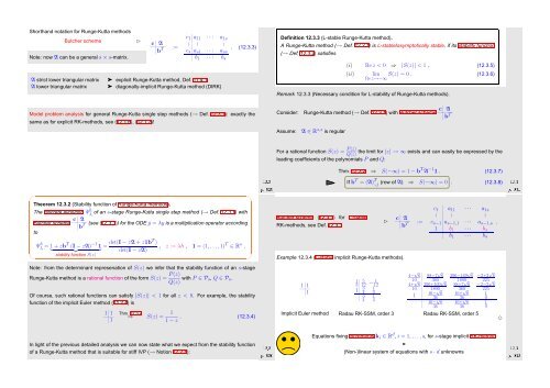
Example 12.3.4 (L-stable implicit Runge-Kutta methods).
c 1 a 11 · · · a 1s
. .
.
c s−1 a s−1,1 · · · a s−1,s .
b 1 · · · b s
1 b 1 · · · b s
△
Note: from the determinant represenation of S(z) we infer that the stability function of an s-stage
Runge-Kutta method is a rational function of the form S(z) = P(z)
Q(z) with P ∈ P s, Q ∈ P s .
Of course, such rational functions can satisfy |S(z)| < 1 for all z < 0. For example, the stability
function of the implicit Euler method (11.2.4) is
1 1
1
Thm. 12.3.2
⇒ S(z) = 1
1 − z . (12.3.4)
1 1
1
1 5
3 12 −12
1
1 3 1
4 4
3 1
4 4
4− √ 6 88−7 √ 6 296−169 √ 6 −2+3 √ 6
10 360 1800 225
4+ √ 6 296+169 √ 6 88+7 √ 6 −2−3 √ 6
10 1800 360 225
16− √ 6 16+ √ 6
1
1
36 36 9
16− √ 6 16+ √ 6 1
36 36 9
Implicit Euler method Radau RK-SSM, order 3 Radau RK-SSM, order 5
✸
In light of the previous detailed analysis we can now state what we expect from the stability function
of a Runge-Kutta method that is suitable for stiff IVP (→ Notion 12.2.1):
Ôº¿¼ ½¾º¿
Equations fixing increments k i ∈ R d , i = 1, ...,s, for s-stage implicit RK-method
=
(Non-)linear system of equations with s · d unknowns
Ôº¿¾ ½¾º¿