Numerical Methods Contents - SAM

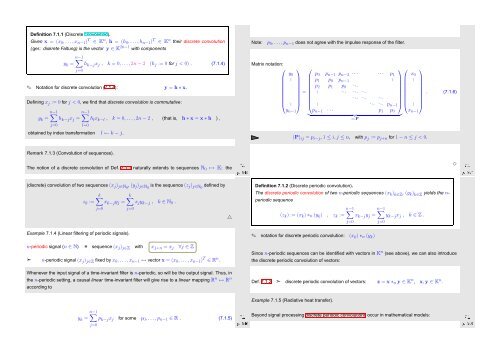
Definition 7.1.1 (Discrete convolution).
Given x = (x 0 , ...,x n−1 ) T ∈ K n , h = (h 0 ,...,h n−1 ) T ∈ K n their discrete convolution
(ger.: diskrete Faltung) is the vector y ∈ K 2n−1 with components
n−1 ∑
y k = h k−j x j , k = 0, ...,2n − 2 (h j := 0 for j < 0) . (7.1.4)
j=0
✎ Notation for discrete convolution (7.1.4): y = h ∗ x.
Defining x j := 0 for j < 0, we find that discrete convolution is commutative:
n−1 ∑ n−1 ∑
y k = h k−j x j = h l x k−l , k = 0, ...,2n − 2 , (that is, h ∗ x = x ∗ h ) ,
j=0
l=0
obtained by index transformation l ← k − j.
Remark 7.1.3 (Convolution of sequences).
The notion of a discrete convolution of Def. 7.1.1 naturally extends to sequences N 0 ↦→ K: the
Ôº º½
Note:
p 0 , ...,p n−1 does not agree with the impulse response of the filter.
Matrix notation:
⎛ ⎞ ⎛
⎞⎛
⎞
y 0 p 0 p n−1 p n−2 · · · · · · p 1 x 0
⎜ ⎜⎜⎜⎜⎜⎜⎜⎝ .
p 1 p 0 p n−1 .
.
p 2 p 1 p . 0
..
=
. ... . .. . ..
. (7.1.6)
. .. . .. . ..
⎟ ⎜
. ⎠ ⎝ . . .. .
⎟⎜
⎟
.. p n−1 ⎠⎝
. ⎠
y n−1 p n−1 · · · p 1 p 0 x n−1
} {{ }
=:P
(P) ij = p i−j , 1 ≤ i,j ≤ n, with p j := p j+n for 1 − n ≤ j < 0.
Ôº º½ ✸
(discrete) convolution of two sequences (x j ) j∈N0 , (y j ) j∈N0 is the sequence (z j ) j∈N0 defined by
z k :=
k∑
x k−j y j =
j=0
Example 7.1.4 (Linear filtering of periodic signals).
k∑
x j y k−j , k ∈ N 0 .
n-periodic signal (n ∈ N) = sequence (x j ) j∈Z with x j+n = x j ∀j ∈ Z
➣ n-periodic signal (x j ) j∈Z fixed by x 0 ,...,x n−1 ↔ vector x = (x 0 , ...,x n−1 ) T ∈ R n .
j=0
Whenever the input signal of a time-invariant filter is n-periodic, so will be the output signal. Thus, in
the n-periodic setting, a causal linear time-invariant filter will give rise to a linear mapping R n ↦→ R n
according to
△
Definition 7.1.2 (Discrete periodic convolution).
The discrete periodic convolution of two n-periodic sequences (x k ) k∈Z , (y k ) k∈Z yields the n-
periodic sequence
n−1 ∑ n−1 ∑
(z k ) := (x k ) ∗ n (y k ) , z k := x k−j y j = y k−j x j , k ∈ Z .
j=0
✎ notation for discrete periodic convolution: (x k ) ∗ n (y k )
Since n-periodic sequences can be identified with vectors in K n (see above), we can also introduce
the discrete periodic convolution of vectors:
Def. 7.1.2 ➣ discrete periodic convolution of vectors: z = x ∗ n y ∈ K n , x,y ∈ K n .
j=0
Ôº º½
n−1 ∑
y k = p k−j x j for some p 0 ,...,p n−1 ∈ R . (7.1.5)
j=0
Example 7.1.5 (Radiative heat transfer).
Beyond signal processing discrete periodic convolutions occur in mathematical models:
Ôº º½