Numerical Methods Contents - SAM

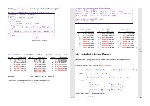
Since lim h→0 T(h) = f ′ (x) ➙ estimate of f ′ (x) by interpolation of T in points h i .
MATLAB-CODE : Numeric differentiation through interpolation with Aitken Neville scheme: nodes x ± h0/2i .
function d = diffex(f,x,h0,tol)
h = h0;
y(1) = (f(x+h0)-f(x-h0))/(2*h0);
for i=2:10
h(i) = h(i-1)/2;
y(i) = (f(x+h(i))-f(x-h(i)))/h(i-1);
for k=i-1:-1:1
y(k) = y(k+1)-(y(k+1)-y(k))*h(i)/(h(i)-h(k));
end
if (abs(y(2)-y(1)) < tol*abs(y(1))), break; end
end
d = y(1);
A posteriori error estimate
Ôº¿ º¿
MATLAB-CODE : Numeric differentiation through finite differences & relative errors.
x=1.1; h=2.ˆ[-1:-5:-36];
atanerr = abs(dirnumdiff(atan,x,h)-1/(1+xˆ2))*(1+xˆ2);
sqrterr = abs(dirnumdiff(sqrt,x,h)-1/(2*sqrt(x)))*(2*sqrt(x));
experr = abs(dirnumdiff(exp,x,h)-exp(x))/exp(x);
function[df]=dirnumdiff(f,x,h)
df=(f(x+h)-f(x))./h;
end
f(x) = arctan(x)
h Relative error
2 −1 0.20786640808609
2 −6 0.00773341103991
2 −11 0.00024299312415
2 −16 0.00000759482296
2 −21 0.00000023712637
2 −26 0.00000001020730
2 −31 0.00000005960464
2 −36 0.00000679016113
f(x) = √ x
h Relative error
2 −1 0.09340033543136
2 −6 0.00352613693103
2 −11 0.00011094838842
2 −16 0.00000346787667
2 −21 0.00000010812198
2 −26 0.00000001923506
2 −31 0.00000001202188
2 −36 0.00000198842224
f(x) = exp(x)
h Relative error
2 −1 0.29744254140026
2 −6 0.00785334954789
2 −11 0.00024418036620
2 −16 0.00000762943394
2 −21 0.00000023835113
2 −26 0.00000000429331
2 −31 0.00000012467100
2 −36 0.00000495453865 ✸
Ôº º¿
diffex2(@atan,1.1,0.5) diffex2(@sqrt,1.1,0.5)
diffex2(@exp,1.1,0.5)
8.3.4 Newton basis and divided differences
Degree Relative error
0 0.04262829970946
1 0.02044767428982
2 0.00051308519253
3 0.00004087236665
4 0.00000048930018
5 0.00000000746031
6 0.00000000001224
Degree Relative error
0 0.02849215135713
1 0.01527790811946
2 0.00061205284652
3 0.00004936258481
4 0.00000067201034
5 0.00000001253250
6 0.00000000004816
7 0.00000000000021
Degree Relative error
0 0.04219061098749
1 0.02129207652215
2 0.00011487434095
3 0.00000825582406
4 0.00000000589624
5 0.00000000009546
6 0.00000000000002
Drawback of the Lagrange basis: adding another data point affects all basis polynomials!
Alternative, “update friendly” method: Newton basis for P n
➣
n−1 ∏
N 0 (t) := 1 , N 1 (t) := (t − t 0 ) , . .. , N n (t) := (t − t i ) . (8.3.3)
LSE for polynomial interpolation problem in Newton basis:
i=0
advantage: guaranteed accuracy ➙ efficiency
a j ∈ R: a 0 N 0 (t j ) + a 1 N 1 (t j ) + · · · + a n N n (t j ) = y j , j = 0, ...,n .
Comparison: numeric differentiation with finite (forward) differences
➙ cancellation ➙ smaller accuracy.
Ôº º¿
⇔
triangular linear system
⎛
⎞
1 0 · · · 0 ⎛ ⎞ ⎛ ⎞
1 (t 1 − t 0 ) ... .
a 0 y 0
. . ... 0
⎜ a 1
⎟
⎜
⎟
⎝
n−1
⎝
∏ ⎠
. ⎠ = ⎜ y 1
⎟
⎝ . ⎠ .
1 (t n − t 0 ) · · · (t n − t i ) a n y n
i=0
Solution of the system with forward substitution:
a 0 = y 0 ,
Ôº º¿