Numerical Methods Contents - SAM

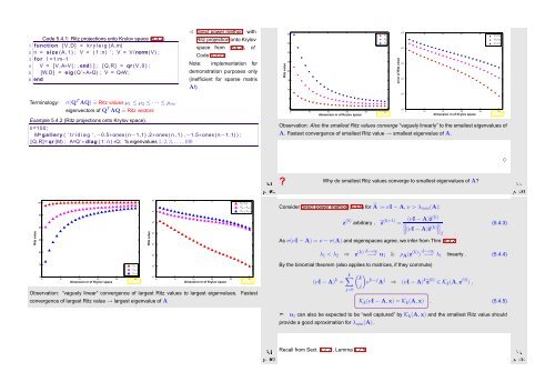
Code 5.4.1: Ritz projections onto Krylov space (5.4.2)
1 function [ V,D] = k r y l e i g (A,m)
2 n = size (A, 1 ) ; V = ( 1 : n ) ’ ; V = V/ norm(V) ;
3 for l =1:m−1
4 V = [ V, A∗V ( : , end ) ] ; [Q,R] = qr (V, 0 ) ;
5 [W,D] = eig (Q’∗A∗Q) ; V = Q∗W;
6 end
✁ direct power method with
Ritz projection onto Krylov
space from (5.4.2), cf.
Code 5.3.21.
Note: implementation for
demonstration purposes only
(inefficient for sparse matrix
A!)
Ritz value
40
35
30
25
20
15
10
µ 1
µ 2
µ 3
error of Ritz value
10 2 dimension m of Krylov space
10 1
10 0
10 −1
|λ 1
−µ 1
|
|λ 2
−µ 2
|
|λ 2
−µ 3
|
10 −2
Terminology: σ(Q T AQ) ˆ= Ritz values µ 1 ≤ µ 2 ≤ · · · ≤ µ m ,
eigenvectors of Q T AQ ˆ= Ritz vectors
Example 5.4.2 (Ritz projections onto Krylov space).
1 n=100;
M= g a llery ( ’ t r i d i a g ’ ,−0.5∗ones ( n−1,1) ,2∗ones ( n , 1 ) ,−1.5∗ones ( n−1,1) ) ;
2 [Q,R]= qr (M) ; A=Q’∗ diag ( 1 : n ) ∗Q; % eigenvalues 1, 2, 3,...,100
5
0
10 −3
5 10 25 5 10 15 20 25 30
15 20
dimension m of Krylov space
30
Fig. 75
Observation: Also the smallest Ritz values converge “vaguely linearly” to the smallest eigenvalues of
A. Fastest convergence of smallest Ritz value → smallest eigenvalue of A.
Fig. 76
Ôº½ º
✸
Ôº¿ º
?
Why do smallest Ritz values converge to smallest eigenvalues of A?
100
10 1
|λ m
−µ m
|
|λ m−1
−µ m−1
|
|λ m−2
−µ m−2
|
Consider direct power method (5.3.5) for à := νI − A, ν > λ max(A):
Ritz value
95
90
85
Ritz value
10 2
10 0
10 −1
10 −2
dimension m of Krylov space
z (0) arbitrary , ˜z (k+1) (νI − A)˜z(k)
=
∥
∥
∥(νI − A)˜z (k) (5.4.3)
∥∥2
As σ(νI − A) = ν − σ(A) and eigenspaces agree, we infer from Thm. 5.3.2
80
10 −3
λ 1 < λ 2 ⇒ z (k) k→∞
−→ u 1
& ρ A (z (k) ) k→∞ −→ λ 1 linearly . (5.4.4)
75
70
5 10 15 20 25 30
dimension m of Krylov space
µ m
µ m−1
µ m−2
Fig. 73
10 −4
10 −5
5 10 15 20 25 30
Observation: “vaguely linear” convergence of largest Ritz values to largest eigenvalues. Fastest
convergence of largest Ritz value → largest eigenvalue of A
Fig. 74
By the binomial theorem (also applies to matrices, if they commute)
(νI − A) k =
k∑
j=0
( k
j)
ν k−j A j ⇒ (νI − A) k˜z (0) ∈ K k (A,z (0) ) ,
K k (νI − A,x) = K k (A,x) . (5.4.5)
Ôº¾ º
➣ u 1 can also be expected to be “well captured” by K k (A,x) and the smallest Ritz value should
provide a good aproximation for λ min (A).
Recall from Sect. 4.2.2 , Lemma 4.2.5:
Ôº º