Numerical Methods Contents - SAM

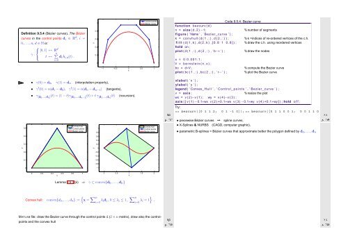
Definition 9.5.4 (Bézier curves). The Bézier
curves in the control points d i ∈ R d , i =
0,...,n, d ∈ N is:
⎧
⎨ [0, 1] ↦→ R d
γ : ∑
⎩ t ↦→
n d i b i,n (t) .
i=0
0.5
0.4
• γ(0) = d 0 , γ(1) = d n (interpolation property),
• γ ′ (0) = n(d 1 − d 0 ), γ ′ (1) = n(d n − d n−1 ) (tangents),
y
1
0.8
0.6
0.4
0.2
0
Control points
Bezier curve
−1 −0.5 0 0.5 1
x
• γ [d0 ,...,d n ] (t) = (1 − t)γ [d 0 ,...,d n−1 ] (t) + t γ [d 1 ,...,d n ](t) (recursion).
Convex hull
Control points
Bezier curve
1
0.8
0.6
Convex hull
Control points
Bezier curve
Ôº º
1 function bezcurv ( d )
Code 9.5.4: Bezier curve
2 n = size ( d , 2 ) −1; % number of segments
3 figure ( ’Name ’ , ’ Bezier curve ’ ) ;
4 k = convhull ( d ( 1 , : ) , d ( 2 , : ) ) ; % k =indices of re-ordered vertices of the c.h.
5 f i l l ( d ( 1 , k ) , d ( 2 , k ) , [ 0 . 8 1 0 . 8 ] ) ; % draw the c.h. using reordered vertices
6 hold on ;
7 plot ( d ( 1 , : ) , d ( 2 , : ) , ’ b−∗ ’ ) ; % draw the nodes
8
9 x = 0 : 0 . 0 0 1 : 1 ;
10 V = b e r n s t e i n ( n , x ) ;
11 bc = d∗V ; % compute the Bezier curve
12 plot ( bc ( 1 , : ) , bc ( 2 , : ) , ’ r−’ ) ; % plot the Bezier curve
13
14 xlabel ( ’ x ’ ) ;
15 ylabel ( ’ y ’ ) ;
16 legend ( ’ Convex H u l l ’ , ’ C o n trol p o i n t s ’ , ’ Bezier curve ’ ) ;
17 v = axis ; % resize the plot
18 wx = v ( 2 )−v ( 1 ) ; wy = v ( 4 )−v ( 3 ) ;
19 axis ( [ v ( 1 ) −0.1∗wx v ( 2 ) +0.1∗wx v ( 3 ) −0.1∗wy v ( 4 ) +0.1∗wy ] ) ; hold o f f ;
Try:
Ôº º
>> bezcurv([0 1 1 2; 0 1 -1 0]); >> bezcurv([0 1 1 0 0 1; 0 0 1 1 0 0]);
• piecewise Bézier curves ➙ spline curves,
• X-Splines & NURBS
(CAGD, computer graphic),
• parametric B-splines = Bézier curves that approximate better the polygon defined by d 0 , ...,d n
0.4
0.3
0.2
y
y
0
0.2
−0.2
−0.4
0.1
−0.6
−0.8
0
−1
0 0.2 0.4 0.6 0.8 1
x
0 0.5 1 1.5 2
x
Lemma 9.5.3 (ii) ⇒ γ ⊂ convex{d 0 , . ..,d n }
Convex hull: convex{d 0 ,...,d n } :=
{x = ∑ n
i=0 λ id i , 0 ≤ λ i ≤ 1, ∑ n }
i=0 λ i = 1 .
MATLAB file: draw the Bezier curve through the control points d (2 × n matrix), draw also the controlpoints
and the convex hull
Ôº º
Ôº¼ º