Numerical Methods Contents - SAM

9.1 Shape preserving interpolation
y
y
When reconstructing a quantitative dependence of quantities from measurements, first principles from
physics often stipulated qualitative constraints, which translate into shape properties of the function
f, e.g., when modelling the material law for a gas:
t i pressure values, y i densities ➣ f positive & monotone.
Given data: (t i , y i ) ∈ R 2 , i = 0, ...,n, n ∈ N, t 0 < t 1 < · · · < t n .
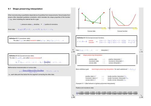
Convex data
Fig. 104t
Convex function
Fig. 105t
Definition 9.1.1 (monotonic data).
The data (t i ,y i ) are called monotonic when y i ≥ y i−1 or y i ≤ y i−1 , i = 1, ...,n.
Ôº º½
Definition 9.1.3 (Convex/concave function).
f : I ⊂ R ↦→ R
convex
concave
:⇔
f(λx + (1 − λ)y) ≤ λf(x) + (1 − λ)f(y)
f(λx + (1 − λ)y) ≥ λf(x) + (1 − λ)f(y)
∀ 0 ≤ λ ≤ 1 ,
∀ x,y ∈ I .
Ôº½ º½
Data (t i ,y i ), i = 0,...,n −→ interpolant f
Definition 9.1.2 (Convex/concave data).
The data {(t i , y i )} n i=0 are called convex (concave) if
∆ j
(≥)
≤ ∆ j+1 , j = 1,...,n − 1 , ∆ j := y j − y j−1
t j − t j−1
, j = 1,...,n .
Mathematical characterization of convex data:
y i ≤ (t i+1 − t i )y i−1 + (t i − t i−1 )y i+1
t i+1 − t i−1
∀ i = 1, ...,n − 1,
i.e., each data point lies below the line segment connecting the other data.
✬
Goal:
✫
shape preserving interpolation:
positive data −→ positive interpolant f,
monotonic data −→ monotonic interpolant f,
convex data −→ convex interpolant f.
More ambitious goal: local shape preserving interpolation: for each subinterval I = (t i , t i+j )
positive data in I −→ locally positive interpolant f| I ,
monotonic data in I −→ locally monotonic interpolant f| I ,
convex data in I −→ locally convex interpolant f| I .
Example 9.1.1 (Bad behavior of global polynomial interpolants).
✩
✪
Ôº¼ º½
Positive and monotonic data:
t i -1.0000 -0.6400 -0.3600 -0.1600 -0.0400 0.0000 0.0770 0.1918 0.3631 0.6187 1.0000
y i
Ôº¾ º½
0.0000 0.0000 0.0039 0.1355 0.2871 0.3455 0.4639 0.6422 0.8678 1.0000 1.0000