Numerical Methods Contents - SAM

Illustration: columns = ONB of Im(A) rows = ONB of Ker(A)
⎛ ⎞ ⎛
⎞⎛
⎞
Σ r 0
⎛ ⎞
A
=
U
⎜ V ⎝
⎟
⎠ (5.5.4)
0 0
⎜ ⎟ ⎜
⎟⎜
⎟
⎝ ⎠ ⎝
⎠⎝
⎠
12 colormap ( cool ) ; view (35 ,10) ;
13
14 p r i n t −depsc2 ’ . . / PICTURES/ svdpca . eps ’ ;
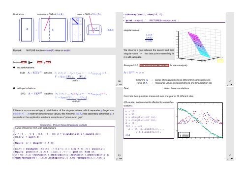
singular values:
3.1378
1.8092
0.1792
0.2
0
−0.2
−0.4
−0.6
−0.8
−1
Remark: MATLAB function r=rank(A) relies on svd(A)
Lemma 5.5.4 PCA by SVD
➊ no perturbations:
We observe a gap between the second and third
singular value ➣ the data points essentially lie
in a 2D subspace.
−1.2
−1.4
−1.6
−1.8
−1
−0.5
0
Example 5.5.5 (Principal component analysis for data analysis).
0.5
1
1.5 −0.5
0
0.5
1
1.5
Fig. 85
SVD: A = UΣV H satisfies σ 1 ≥ σ 2 ≥ ...σ p > σ p+1 = · · · = σ min{m,n} = 0 ,
V = Span {(U) :,1 ,...,(U) :,p } .
} {{ }
ONB of V
Ôº º
A ∈ R m,n , m ≫ n:
Columns A → series of measurements at different times/locations etc.
➋
with perturbations:
Rows of A → measured values corresponding to one time/location etc.
Ôº½
º
Goal:
detect linear correlations
SVD: A = UΣV H satisfies σ 1 ≥ σ 2 ≥ . ..σ p ≫σ p+1 ≈ · · · ≈ σ min{m,n} ≈ 0 ,
V = Span {(U) :,1 , ...,(U) :,p } .
} {{ }
ONB of V
If there is a pronounced gap in distribution of the singular values, which separates p large from
min{m, n} − p relatively small singular values, this hints that Im(A) has essentially dimension p. It
depends on the application what one accepts as a “pronounced gap”.
Code 5.5.4: PCA in three dimensions via SVD
1 % Use of SVD for PCA with perturbations
2
3 V = [1 , −1; 0 , 0 . 5 ; −1 , 0 ] ; A = V∗rand ( 2 ,20) +0.1∗rand ( 3 ,20) ;
4 [U, S, V] = svd (A, 0 ) ;
5
Ôº¼ º
11 mesh( reshape (M( 1 , : ) ,n ,m) , reshape (M( 2 , : ) ,n ,m) , reshape (M( 3 , : ) ,n ,m) ) ;
6 figure ; sv = diag (S( 1 : 3 , 1 : 3 ) )
7
8 [ X, Y ] = meshgrid ( −2:0.2:0 , −1:0.2:1) ; n = size (X, 1 ) ; m = size (X, 2 ) ;
9 figure ; plot3 (A ( 1 , : ) ,A ( 2 , : ) ,A ( 3 , : ) , ’ r ∗ ’ ) ; grid on ; hold on ;
10 M = U( : , 1 : 2 ) ∗[ reshape (X, 1 , prod ( size (X) ) ) ; reshape (Y, 1 , prod ( size (Y) ) ) ] ;
Concrete: two quantities measured over one year at 10 different sites
(Of course, measurements affected by errors/fluctuations)
n = 10;
m = 50;
x = sin(pi*(1:m)’/m);
y = cos(pi*(1:m)’/m);
A = [];
for i = 1:n
A = [A, x.*rand(m,1),...
y+0.1*rand(m,1)];
end
1.5
1
0.5
0
−0.5
measurement 1
measurement 2
measurement 2
measurement 4
−1
0 5 10 15 20 25 30 35 40 45 50
Ôº¾ º