Numerical Methods Contents - SAM

y i+1
t i−1 t i t i+1
y i−1
y i
y i−1
y i−1
y i
y i+1
y i+1 y i
t i−1 t i t i+1 t i−1 t i t i+1
➁ Choice of “middle points” p i ∈ (t i−1 ,t i ], i = 1,...,n:
⎧
intersection of the two straight lines
⎪⎨
resp. through (t
p i =
i−1 ,y i−1 ), (t i , y i ) if the intersection point belongs to (t i−1 , t i ] ,
with slopes c i−1 ,c i ⎪⎩ 1
2 (t i−1 + t i ) otherwise .
This points will be used to build the grid for the final quadratic spline:
M = {t 0 < p 1 ≤ t 1 < p 2 ≤ · · · < p n ≤ t n }.
Ôº¿ º
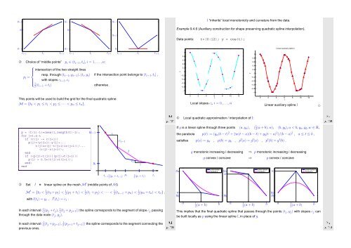
l “inherits” local monotonicity and curvature from the data.
Example 9.4.6 (Auxiliary construction for shape preserving quadratic spline interpolation).
Data points: t=(0:12); y = cos(t);
y
1
0.8
0.6
0.4
0.2
0
−0.2
−0.4
−0.6
−0.8
−1
0 2 4 6 8 10 12
t
Local slopes c i , i = 0, ...,n
y
Linear auxiliary spline l
1
0.8
0.6
0.4
0.2
0
−0.2
−0.4
−0.6
−0.8
−1
0 2 4 6 8 10 12
t
Ôº¿ º
➃ Local quadratic approximation / interpolation of l:
Linear auxiliary spline l
✸
If g is a linear spline through three points (a,y a ), ( 1 2 (a + b), w), (b, y b), a < b, y a ,y b , w ∈ R,
p = (t(1)-1)*ones(1,length(t)-1);
for j=1:n-1
if (c(j) ~= c(j+1))
p(j)=(y(j+1)-y(j)+...
t(j)*c(j)-t(j+1)*c(j+1))/...
(c(j)-c(j+1));
end
if ((p(j)t(j+1)))
p(j) = 0.5*(t(j)+t(j+1));
end;
end
y i−1
y i
t i−1
1
c i−1
l
1
2 (p i + t i−1 )
p i
c i
1
1
2 (p i + t i )
t i
the parabola p(t) := (y a (b − t) 2 + 2w(t − a)(b − t) + y b (t − a) 2 )/(b − a) 2 , a ≤ t ≤ b ,
satisfies p(a) = y a , p(b) = y b , p ′ (a) = g ′ (a) , p ′ (b) = g ′ (b) .
g monotonic increasing / decreasing ⇒ p monotonic increasing / decreasing
g convex / concave ⇒ p convex / concave
y a
Linear Spline l
Parabola p
y a
w
Linear Spline l
Parabola p
w
Linear Spline l
Parabola p
➂ Set l = linear spline on the mesh M ′ (middle points of M)
M ′ = {t 0 < 1 2 (t 0 + p 1 ) < 1 2 (p 1 + t 1 ) < 1 2 (t 1 + p 2 ) < · · · < 1 2 (t n−1 + p n ) < 1 2 (p n + t n ) < t n } ,
with l(t i ) = y i , l ′ (t i ) = c i .
In each interval ( 1 2 (p j + t j ), 1 2 (t j + p j+1 )) the spline corresponds to the segment of slope c j passing
through the data node (t j , y j ).
In each interval ( 1 2 (t j +p j+1 ), 1 2 (p j+1 +t j+1 )) the spline corresponds to the segment connecting the
previous ones.
Ôº¿ º
w
y b
a
1
2 (a + b)
b
y b
a
1
2 (a + b)
b
y a
yb
a
1
2 (a + b)
This implies that the final quadratic spline that passes through the points (t j ,y j ) with slopes c j can
be built locally as p using the linear spline l, in place of g.
b
Ôº¼ º