Numerical Methods Contents - SAM

0
0
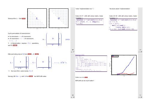
“naive” implementation via “\”:
“structure aware” implementation:
2
2
Obvious fill-in (→ Def. 2.6.3)
4
6
L
8
10
12
0 2 4 6 8 10 12
nz = 65
4
6
U
8
10
12
0 2 4 6 8 10 12
nz = 65
Code 2.6.17: LSE with arrow matrix, implementation
I
1 function x = sa1 ( alpha , b , c , d , y )
2 A = [ alpha , b ’ ; c , diag ( d ) ] ;
3 x = A \ y ;
Code 2.6.19: LSE with arrow matrix, implementation
II
1 function x = sa2 ( alpha , b , c , d , y )
2 z = b . / d ;
3 x i = ( y ( 1 ) −
dot ( z , y ( 2 : end ) ) ) . . .
4 / ( alpha−dot ( z , c ) ) ;
5 x = [ x i ; ( y ( 2 : end )−x i ∗c ) . / d ] ;
Cyclic permutation of rows/columns:
• 1st row/column → n-th row/column
• i-th row/column → i − 1-th row/column,
i = 2,...,n
➣
LU-factorization requires O(n) operations,
see Ex. 2.6.13.
⎛
A =
⎜
⎝
D
b T
⎞
c
⎟
⎠
α
(2.6.2)
Ôº½ ¾º
Ôº½ ¾º
After permuting rows of A from (2.6.2) , cf. (2.2.2):
⎛
⎞ ⎛
L =
I 0
, U =
⎜
⎟ ⎜
⎝
⎠ ⎝
b T D −1 1
➣ No more fill-in, costs merely O(n) !
⎞
D c
, σ := α − b T D −1 c .
⎟
⎠
0 σ
Measuring run times:
t = [];
for i=3:12
n = 2^n; alpha = 2;
b = ones(n,1); c = (1:n)’;
d = -ones(n,1); y = (-1).^(1:(n+1))’;
tic; x1 = sa1(alpha,b,c,d,y); t1 = toc;
tic; x2 = sa2(alpha,b,c,d,y); t2 = toc;
t = [t; n t1 t2];
end
loglog(t(:,1),t(:,2), ...
... ’b-*’,t(:,1),t(:,3),’r-+’);
time[seconds]
10 1
10 0
10 −1
10 −2
10 −3
Implementation I
Implementation II
Solving LSE Ax = y with A from 2.6.1:
two MATLAB codes
Platform as in Ex. 2.6.5
10 2 n
10 −4
10 0 10 1 10 2 10 3 10 4
MATLAB can do much better !
Ôº½ ¾º
Ôº½¼ ¾º