Numerical Methods Contents - SAM

|quadrature error|
10 0 Numerical quadrature of function 1/(1+(5t) 2 )
10 −2
10 −4
10 −6
10 −8
10 −10
10 −12
10 −14
Equidistant Newton−Cotes quadrature
Chebyshev quadrature
Gauss quadrature
0 2 4 6 8 10 12 14 16 18 20
Number of quadrature nodes
10 0 Numerical quadrature of function sqrt(t)
2 on [0, 1] quadrature error, f 1 (t) := 1
1+(5t) quadrature error, f 2 (t) := √ t on [0, 1]
10 0 10 1
Number of quadrature nodes
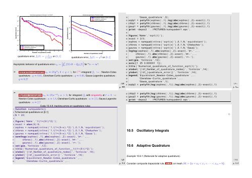
Asymptotic behavior of quadrature error ǫ n := ∣ ∫ 1
0 f(t) dt − Q n (f) ∣ for "‘n → ∞”:
➣
|quadrature error|
10 −1
10 −2
10 −3
10 −4
10 −5
10 −6
Equidistant Newton−Cotes quadrature
Chebyshev quadrature
Gauss quadrature
exponential convergence ǫ n ≈ O(q n ), 0 < q < 1, for C ∞ -integrand f 1 ❀ : Newton-Cotes
quadrature : q ≈ 0.61, Clenshaw-Curtis quadrature : q ≈ 0.40, Gauss-Legendre quadrature :
q ≈ 0.27
Ôº¼ ½¼º
19 ’ Gauss quadrature ’ ,3) ;
20 eqdp1 = p o l y f i t ( eqdres ( : , 1 ) , log ( abs ( eqdres ( : , 2 )−exact ) ) ,1)
21 chbp1 = p o l y f i t ( chbres ( : , 1 ) , log ( abs ( chbres ( : , 2 )−exact ) ) ,1)
22 gaup1 = p o l y f i t ( gaures ( : , 1 ) , log ( abs ( gaures ( : , 2 )−exact ) ) ,1)
23 p r i n t −depsc2 ’ . . / PICTURES/ numquaderr1 . eps ’ ;
24
25 figure ( ’Name ’ , ’ s q r t ( t ) ’ ) ;
26 exact = 2 / 3 ;
27 eqdres = numquad( i n l i n e ( ’ s q r t ( x ) ’ ) ,0 ,1 ,N, ’ e q u i d i s t a n t ’ ) ;
28 chbres = numquad( i n l i n e ( ’ s q r t ( x ) ’ ) ,0 ,1 ,N, ’ Chebychev ’ ) ;
29 gaures = numquad( i n l i n e ( ’ s q r t ( x ) ’ ) ,0 ,1 ,N, ’ Gauss ’ ) ;
30 loglog ( eqdres ( : , 1 ) , abs ( eqdres ( : , 2 )−exact ) , ’ b+− ’ , . . .
31 chbres ( : , 1 ) ,abs ( chbres ( : , 2 )−exact ) , ’m+− ’ , . . .
32 gaures ( : , 1 ) ,abs ( gaures ( : , 2 )−exact ) , ’ r+− ’ ) ;
33 set ( gca , ’ f o n t s i z e ’ ,12) ;
34 axis ( [ 1 25 0.000001 1 ] ) ;
35 t i t l e ( ’ Numerical quadrature o f f u n c t i o n s q r t ( t ) ’ ) ;
36 xlabel ( ’ { \ b f Number o f quadrature nodes } ’ , ’ f o n t s i z e ’ ,14) ;
37 ylabel ( ’ { \ b f | quadrature e r r o r | } ’ , ’ f o n t s i z e ’ ,14) ;
38 legend ( ’ E q u i d i s t a n t Newton−Cotes quadrature ’ , . . .
39 ’ Clenshaw−C u r t i s quadrature ’ , . . .
40 ’ Gauss quadrature ’ ,1) ;
Ôº½½ ½¼º
41 eqdp2 = p o l y f i t ( log ( eqdres ( : , 1 ) ) , log ( abs ( eqdres ( : , 2 )−exact ) ) ,1)
➣
algebraic convergence ǫn ≈ O(n −α ), α > 0, for integrand f 2 with singularity at t = 0 ❀
Newton-Cotes quadrature : α ≈ 1.8, Clenshaw-Curtis quadrature : α ≈ 2.5, Gauss-Legendre
quadrature : α ≈ 2.7
Code 10.4.8: tracking errors on quadrature rules
1 function numquaderrs ( )
2 % Numerical quadrature on [0,1]
3 N = 20;
4
5 figure ( ’Name ’ , ’ 1 /(1+(5 t ) ^2) ’ ) ;
6 exact = atan ( 5 ) / 5 ;
42 chbp2 = p o l y f i t ( log ( chbres ( : , 1 ) ) , log ( abs ( chbres ( : , 2 )−exact ) ) ,1)
43 gaup2 = p o l y f i t ( log ( gaures ( : , 1 ) ) , log ( abs ( gaures ( : , 2 )−exact ) ) ,1)
44 p r i n t −depsc2 ’ . . / PICTURES/ numquaderr2 . eps ’ ;
✸
7 eqdres = numquad( i n l i n e ( ’ 1 . / ( 1 + ( 5∗ x ) . ^ 2 ) ’ ) ,0 ,1 ,N, ’ e q u i d i s t a n t ’ ) ;
8 chbres = numquad( i n l i n e ( ’ 1 . / ( 1 + ( 5∗ x ) . ^ 2 ) ’ ) ,0 ,1 ,N, ’ Chebychev ’ ) ;
9 gaures = numquad( i n l i n e ( ’ 1 . / ( 1 + ( 5∗ x ) . ^ 2 ) ’ ) ,0 ,1 ,N, ’ Gauss ’ ) ;
10 semilogy ( eqdres ( : , 1 ) ,abs ( eqdres ( : , 2 )−exact ) , ’ b+− ’ , . . .
11 chbres ( : , 1 ) ,abs ( chbres ( : , 2 )−exact ) , ’m+− ’ , . . .
12 gaures ( : , 1 ) ,abs ( gaures ( : , 2 )−exact ) , ’ r+− ’ ) ;
13 set ( gca , ’ f o n t s i z e ’ ,12) ;
14 t i t l e ( ’ Numerical quadrature o f f u n c t i o n 1 /(1+(5 t ) ^2) ’ ) ;
15 xlabel ( ’ { \ b f Number o f quadrature nodes } ’ , ’ f o n t s i z e ’ ,14) ;
16 ylabel ( ’ { \ b f | quadrature e r r o r | } ’ , ’ f o n t s i z e ’ ,14) ;
17 legend ( ’ E q u i d i s t a n t Newton−Cotes quadrature ’ , . . .
18 ’ Clenshaw−C u r t i s quadrature ’ , . . .
Ôº½¼ ½¼º
10.5 Oscillatory Integrals
10.6 Adaptive Quadrature
Example 10.6.1 (Rationale for adaptive quadrature).
Consider composite trapezoidal rule (10.3.2) on mesh M := {a = x 0 < x 1 < · · · < x m = b}:
Ôº½¾ ½¼º