Numerical Methods Contents - SAM

Heuristics: the timestep h is small ➥ “higher order terms” O(h p+2 ) can be ignored.
✎
Ψ h ky(t k ) − Φ h . ky(t k ) = ch p+1
k + O(h p+2
k ) ,
˜Ψ hk y(t k ) − Φ h . ky(t k ) = O(h p+2
k ) .
.
notation: = equality up to higher order terms in h k
⇒ EST k
.
= ch p+1
k . (11.5.6)
• line 9: compute presumably better local stepsize according to (11.5.9),
• line 10: decide whether to repeat the step or advance,
• line 11: extend output arrays if current step has not been rejected.
.
EST k = ch p+1
k ⇒ c = . EST k
h p+1 . (11.5.7)
k
△
Available in algorithm, see (11.5.3)
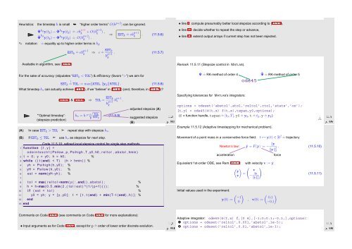
Remark 11.5.11 (Stepsize control in MATLAB).
For the sake of accuracy (stipulates “EST k < TOL”) & efficiency (favors “>”) we aim for
EST k
!
= TOL := max{ATOL, ‖y k ‖RTOL} . (11.5.8)
Ψ ˆ= RK-method of order 4 ˜Ψ ˆ= RK-method of order 5
ode45
What timestep h ∗ can actually achieve (11.5.8), if we “believe” in (11.5.6) (and, therefore, in (11.5.7))?
"‘Optimal timestep”:
(stepsize prediction)
(11.5.7) & (11.5.8) ⇒ TOL = EST k
h p+1
k
h p+1
∗ .
h ∗ = h p+1 √ TOL
EST k
. (11.5.9)
(A): In caseEST k > TOL ➣ repeat step with stepsize h ∗ .
adjusted stepsize (A)
suggested stepsize
(B)
Ôº¿ ½½º
Specifying tolerances for MATLAB’s integrators:
options = odeset(’abstol’,atol,’reltol’,rtol,’stats’,’on’);
[t,y] = ode45(@(t,x) f(t,x),tspan,y0,options);
(f = function handle, tspan ˆ= [t 0 , T], y0 ˆ= y 0 , t ˆ= t k , y ˆ= y k )
Example 11.5.12 (Adaptive timestepping for mechanical problem).
△
Ôº ½½º
(B): IfEST k ≤ TOL ➣ use h ∗ as stepsize for next step.
Movement of a point mass in a conservative force field:
t ↦→ y(t) ∈ R 2 ˆ= trajectory
Code 11.5.10: refined local stepsize control for single step methods
1 function [ t , y ] =
o d e i n t s s c t r l ( Psilow , p , Psihigh , T , y0 , h0 , r e l t o l , abstol , hmin )
2 t = 0 ; y = y0 ; h = h0 ; %
3 while ( ( t ( end ) < T ) ( h > hmin ) ) %
4 yh = Psihigh ( h , y0 ) ; %
5 yH = Psilow ( h , y0 ) ; %
6 est = norm( yH−yh ) ; %
7
8 t o l = max( r e l t o l ∗norm( y ( : , end ) ) , a b s t o l ) ; %
9 h = h∗max( 0 . 5 , min ( 2 , ( t o l / est ) ^ ( 1 / ( p+1) ) ) ) ; %
10 i f ( est < t o l ) %
11 y0 = yh ; y = [ y , y0 ] ; t = [ t , t ( end ) + min ( T−t ( end ) , h ) ] ; %
12 end
13 end
Newton’s law:
acceleration
ÿ = F(y) := − 2y
‖y‖ 2 . (11.5.10)
2
Equivalent 1st-order ODE, see Rem. 11.1.7: with velocity v := ẏ
(ẏ ) ( ) v
=
˙v − 2y . (11.5.11)
‖y‖ 2 2
Initial values used in the experiment:
y(0) :=
( )
−1
0
force
( )
0.1
, v(0) :=
−0.1
Comments on Code 11.5.9 (see comments on Code 11.5.2 for more explanations):
• Input arguments as for Code 11.5.2, except for p ˆ= order of lower order discrete evolution.
Ôº ½½º
Adaptive integrator: ode45(@(t,x) f,[0 4],[-1;0;0.1;-0.1,],options):
➊ options = odeset(’reltol’,0.001,’abstol’,1e-5);
➋ options = odeset(’reltol’,0.01,’abstol’,1e-3);
Ôº ½½º