Numerical Methods Contents - SAM

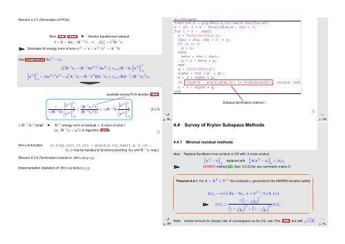
Remark 4.3.7 (Termination of PCG).
Rem. 4.2.3, (4.2.11) ➤ Monitor transformed residual
˜r = ˜b − Øx = B−1/2 r ⇒ ‖˜r‖ 2 2 = rT B −1 r .
Estimates for energy norm of error e (l) := x − x (l) , x ∗ := A −1 b
Use error equation Ae (l) = r l :
r T l B−1 r l = (B −1 Ae (l) ) T Ae (l) ≤ λ max (B −1 ∥
A) ∥e (l)∥ ∥2
, A ∥
∥e (l)∥ ∥2
= A (Ae(l) ) T e (l) = r T l A−1 r l = B −1 r T BA −1 r l ≤ λ max (BA −1 ) (B −1 r l ) T r l .
available during PCG iteration (4.3.2)
MATLAB PCG algorithm
function x = pcg(Afun,b,tol,maxit,Binvfun,x0)
x = x0; r = b - feval(Afun,x); rho = 1;
for i = 1 : maxit
y = feval(Binvfun,r);
rho1 = rho; rho = r’ * y;
if (i == 1)
p = y;
else
beta = rho / rho1;
p = y + beta * p;
end
q = feval(Afun,p);
alpha = rho /(p’ * q);
x = x + alpha * p;
if (norm(b - evalf(Afun,x))