Numerical Methods Contents - SAM

Code 9.3.5: Hermite approximation and orders of convergence with exact slopes
1 % 16.11.2009 hermiteapprox1.m
2 % Plot convergence of approximation error of cubic hermite interpolation
3 % with respect to the meshwidth
4 % print the algebraic order of convergence in sup and L 2 norms
5 % Slopes: exact slopes of f
6 %
7 % inputs: f function to be interpolated
8 % df derivative of f
9 % a, b left and right extremes of the interval
10 % N maximum number of subdomains
11
12 function hermiteapprox1 ( f , df , a , b ,N)
13 e r r = [ ] ;
14 for j =2:N
15 xx=a ; % xx is the mesh on which the error is computed, built in the k-loop
16 v a l = f ( a ) ;
17
Ôº¼ º¿
22 for k =1: j −1
18 t = a : ( b−a ) / j : b ; % nodes
19 y = f ( t ) ;
20 c= d f ( t ) ; % compute exact slopes
21
e xp_rate_Linf= p I ( 1 )
46 pL2 = p o l y f i t ( log ( e r r ( c e i l (N/ 2 ) :N−2,1) ) , log ( e r r ( c e i l (N/ 2 ) :N−2,3) ) ,1) ;
exp_rate_L2=pL2 ( 1 )
47 hold on ;
48 plot ( [ e r r ( 1 , 1 ) , e r r (N−1,1) ] , [ e r r ( 1 , 1 ) , e r r (N−1,1) ] . ^ p I ( 1 ) ∗exp ( p I ( 2 ) ) , ’m ’ )
49 plot ( [ e r r ( 1 , 1 ) , e r r (N−1,1) ] ,
[ e r r ( 1 , 1 ) , e r r (N−1,1) ] . ^ pL2 ( 1 ) ∗exp ( pL2 ( 2 ) ) , ’ k ’ )
Try: hermiteapprox1(@atan, @(x) 1./(1+x.∧2), -5,5,100);
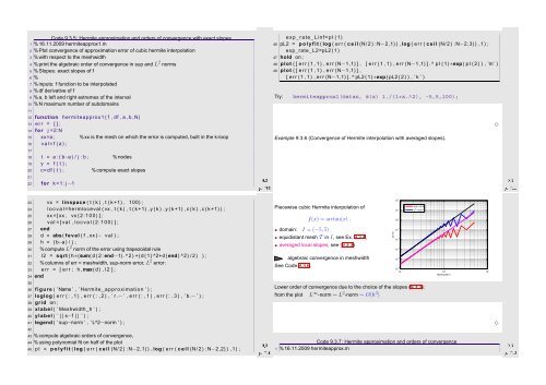
Example 9.3.6 (Convergence of Hermite interpolation with averaged slopes).
✸
Ôº½½ º¿
23 vx = linspace ( t ( k ) , t ( k +1) , 100) ;
24 l o c v a l =hermloceval ( vx , t ( k ) , t ( k +1) , y ( k ) , y ( k +1) , c ( k ) , c ( k +1) ) ;
25 xx =[ xx , vx ( 2 : 1 0 0 ) ] ;
26 v a l =[ val , l o c v a l ( 2 : 1 0 0 ) ] ;
27 end
28 d = abs ( feval ( f , xx )− v a l ) ;
29 h = ( b−a ) / j ;
30 % compute L 2 norm of the error using trapezoidal rule
31 l 2 = sqrt ( h∗(sum( d ( 2 : end−1) . ^ 2 ) +(d ( 1 ) ^2+d ( end ) ^2) / 2 ) ) ;
32 % columns of err = meshwidth, sup-norm error, L 2 error:
33 e r r = [ e r r ; h ,max( d ) , l 2 ] ;
34 end
35
36 figure ( ’Name ’ , ’ Hermite approximation ’ ) ;
37 loglog ( e r r ( : , 1 ) , e r r ( : , 2 ) , ’ r .− ’ , e r r ( : , 1 ) , e r r ( : , 3 ) , ’ b.− ’ ) ;
38 grid on ;
39 xlabel ( ’ Meshwidth h ’ ) ;
40 ylabel ( ’ | | s−f | | ’ ) ;
41 legend ( ’ sup−norm ’ , ’ L^2−norm ’ ) ;
Ôº½¼ º¿
45 p I = p o l y f i t ( log ( e r r ( c e i l (N/ 2 ) :N−2,1) ) , log ( e r r ( c e i l (N/ 2 ) :N−2,2) ) ,1) ;
42
43 % compute algebraic orders of convergence,
44 % using polynomial fit on half of the plot
Piecewise cubic Hermite interpolation of
domain: I = (−5, 5)
f(x) = arctan(x) .
equidistant mesh T in I, see Ex. 9.3.4,
averaged local slopes, see (9.3.3)
algebraic convergence in meshwidth
See Code 9.3.6.
Lower order of convergence due to the choice of the slopes (9.3.3):
from the plot L ∞ -norm ∼ L 2 -norm ∼ O(h 3 )
||s−f||
sup−norm
L 2 −norm
10 2
10 1
10 0
10 −1
10 −2
10 −3
10 −4
10 −5
10 −1 10 0
Meshwidth h
10 1
✸
Ôº½¾ º¿
Code 9.3.7: Hermite approximation and orders of convergence
1 % 16.11.2009 hermiteapprox.m