Numerical Methods Contents - SAM

MATLAB-CODE Sine transform
function s = sinetrans(y)
n = length(y)+1;
sinevals = imag(exp(i*pi/n).^(1:n-1));
yt = [0 (sinevals.*(y+y(end:-1:1)) + 0.5*(y-y(end:-1:1)))];
c = fftreal(yt);
s(1) = dot(sinevals,y);
for k=2:N-1
if (mod(k,2) == 0), s(k) = -imag(c(k/2+1));
else, s(k) = s(k-2) + real(c((k-1)/2+1)); end
end
⎛
⎞
C c y I 0 · · · · · · 0
c y I C c y I .
T =
⎜ 0 . .. ... . ..
⎟
⎝ . c y I C c y I⎠ ∈ Rn2 ,n 2 ,
0 · · · · · · 0 c y I C
⎛
⎞
c c x 0 · · · · · · 0
c x c c x .
C =
⎜ 0 . .. ... ...
⎟
⎝ . c x c c x ⎠ ∈ Rn,n .
0 · · · · · · 0 c x c
j
n+1 n+2
1 2 3
c x
c y
c y
c x
i
△
Application:
diagonalization of local translation invariant linear operators.
5-points-stencil-operator on R n,n , n ∈ N, in grid representation:
T : R n,n ↦→ R n,n ,
X ↦→ T(X)
(T(X)) ij := cx ij + c y x i,j+1 + c y x i,j−1 + c x x i+1,j + c x x i−1,j
Ôº¼ º
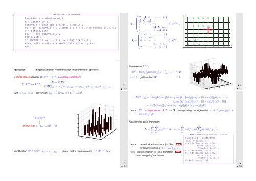
Sine basis of R n,n :
B kl = ( sin( n+1 π ki) sin( π
n+1 lj)) n
i,j=1 . (7.4.2)
n = 10: grid function B 2,3 ➣
1
0.5
0
−0.5
−1
1
2
3
4
10
5
9
6
8
7
7
6
5
8
4
9
3
2
10
1
Ôº½½ º
with c,c y ,c x ∈ R, convention: x ij := 0 for (i,j) ∉ {1,...,n} 2 .
X ∈ R n,n
↕
grid function ∈ {1, . ..,n} 2 ↦→ R
25
20
15
10
5
0
1
2
3
4
5
5
4
3
2
1
(T(B kl )) ij = c sin( n πki) sin(π n lj) + c y sin( π n ki)( sin( n+1 π l(j − 1)) + sin( π
n+1 l(j + 1))) +
c x sin( n πlj)( sin( n+1 π k(i − 1)) + sin( π
n+1k(i + 1)))
= sin( π n ki) sin(π n lj)(c + 2c y cos( n+1 π l) + 2c x cos( n+1 π k))
Hence B kl is eigenvector of T ↔ T corresponding to eigenvalue c + 2c y cos( n+1 π 2c x cos( n+1 π Algorithm for basis transform:
X =
n∑
k=1 l=1
n∑
y kl B kl ⇒ x ij =
n∑
sin( n+1 π ki) ∑ n
k=1 l=1
y kl sin( π
n+1 lj) .
MATLAB-CODE two dimensional sine tr.
Identification R n,n ∼ = R n2 , x ij ∼ ˜x (j−1)n+i gives matrix representation T ∈ R n2 ,n 2 of T :
i
Ôº½¼ º
Hence nested sine transforms (→ Sect. 7.2.4)
for rows/columns of Y = (y kl ) n k,l=1 .
Here: implementation of sine transform (7.4.1)
with “wrapping”-technique.
function C = sinft2d(Y)
[m,n] = size(Y);
C = fft([zeros(1,n); Y;...
zeros(1,n);...
-Y(end:-1:1,:)]);
C = i*C(2:m+1,:)’/2;
C = fft([zeros(1,m); C;...
zeros(1,m);...
Ôº½¾ º
-C(end:-1:1,:)]);
C= i*C(2:n+1,:)’/2;