

Numerical Methods Contents - SAM
Numerical Methods Contents - SAM
Numerical Methods Contents - SAM

Create successful ePaper yourself
Turn your PDF publications into a flip-book with our unique Google optimized e-Paper software.
f<br />
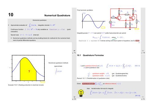
10 <strong>Numerical</strong> Quadrature<br />
<strong>Numerical</strong> quadrature<br />
∫<br />
= Approximate evaluation of f(x) dx, integration domain Ω ⊂ R d<br />
Ω<br />
Continuous function f : Ω ⊂ R d ↦→ R only available as function y = f(x) (point<br />
evaluation)<br />
Special case d = 1: Ω = [a,b] (interval)<br />
☞ <strong>Numerical</strong> quadrature methods are key building blocks for methods for the numerical treatment<br />
of partial differential equations.<br />
Time-harmonic excitation:<br />
U(t)<br />
T t<br />
Fig. 108<br />
R 3 R 4<br />
R 1<br />
➀<br />
➃<br />
R b<br />
➂<br />
➄<br />
➁<br />
R<br />
U(t)<br />
L<br />
R e R<br />
I(t)<br />
2<br />
Fig. 109<br />
Integrating power P = UI over period [0,T] yields heat production per period:<br />
∫ T<br />
W therm = U(t)I(t) dt , where I = I(U) .<br />
0<br />
function I = current(U) involves solving non-linear system of equations, see Ex. 3.0.1!<br />
✸<br />
Ôº½ ½¼º¼<br />
Ôº¿ ½¼º½<br />
3<br />
10.1 Quadrature Formulas<br />
2.5<br />
2<br />
1.5<br />
1<br />
0.5<br />
?<br />
<strong>Numerical</strong> quadrature methods<br />
approximate<br />
∫b<br />
f(t) dt<br />
a<br />
n-point quadrature formula on [a,b]:<br />
(n-point quadrature rule)<br />
∫ b<br />
n∑<br />
f(t) dt ≈ Q n (f) := ωj n f(ξn j ) . (10.1.1)<br />
a<br />
j=1<br />
ω n j : quadrature weights ∈ R (ger.: Quadraturgewichte)<br />
ξ n j : quadrature nodes ∈ [a,b] (ger.: Quadraturknoten)<br />
Remark 10.1.1 (Transformation of quadrature rules).<br />
0<br />
0 0.5 1 1.5 2 2.5 3 3.5 4<br />
t<br />
Fig. 107<br />
Example 10.0.1 (Heating production in electrical circuits).<br />
) n<br />
Given: quadrature formula<br />
(̂ξj , ̂ω j on reference interval [−1, 1]<br />
j=1<br />
Ôº¾ ½¼º¼<br />
Idea: transformation formula for integrals<br />
∫ b<br />
∫ 1<br />
f(t) dt = 1 2 (b − a) a<br />
−1<br />
̂f(τ) dτ , ̂f(τ) := f( 1<br />
2 (1 − τ)a + 1 2 (τ + 1)b) .<br />
Ôº ½¼º½<br />
(10.1.2)


