Numerical Methods Contents - SAM

Note: sensitivity gauge depends on the chosen norm !
Example 2.5.11 (Intersection of lines in 2D).
In distance metric:
2.6 Sparse Matrices
A classification of matrices:
Dense matrices (ger.: vollbesetzt)
sparse matrices (ger.: dünnbesetzt)
nearly orthogonal intersection: well-conditioned
glancing intersection: ill-conditioned
Notion 2.6.1 (Sparse matrix). A ∈ K m,n , m, n ∈ N, is sparse, if
nnz(A) := #{(i,j) ∈ {1, . ..,m} × {1, ...,n}: a ij ≠ 0} ≪ mn .
Sloppy parlance: matrix sparse :⇔ “almost all” entries = 0 /“only a few percent of” entries ≠ 0
Hessian normal form of line #i, i = 1, 2:
L i = {x ∈ R 2 : x T n i = d i } , n i ∈ R 2 , d i ∈ R .
( ) ( )
n T
intersection: 1 d1
n
} {{ T x = ,
d
2 2
} } {{ }
=:A =:b
n i ˆ= (unit) direction vectors, d i ˆ= distance to origin.
Ôº½¿ ¾º
A more rigorous “mathematical” definition:
Definition 2.6.2 (Sparse matrices).
Given a strictly increasing sequences m : N ↦→ N, n : N ↦→ N, a family (A (l) ) l∈N of matrices
with A (l) ∈ K m l,n l is sparse (opposite: dense), if
nnz(A (l) ) := #{(i,j) ∈ {1, ...,m i } × {1, ...,n i }: a (l)
Ôº½¿ ¾º
ij ≠ 0} = O(n i + m i ) for i → ∞ .
Code 2.5.12: condition numbers of 2 × 2 matrices
1 r = [ ] ;
2 for phi=pi / 2 0 0 : pi / 1 0 0 : pi /2
3 A = [ 1 , cos ( phi ) ; 0 , sin ( phi ) ] ;
4 r = [ r ; phi ,
cond (A) ,cond (A, ’ i n f ’ ) ] ;
5 end
6 plot ( r ( : , 1 ) , r ( : , 2 ) , ’ r−’ ,
r ( : , 1 ) , r ( : , 3 ) , ’ b−−’ ) ;
7 xlabel ( ’ { \ b f angle o f n_1 ,
n_2 } ’ , ’ f o n t s i z e ’ ,14) ;
8 ylabel ( ’ { \ b f c o n d i t i o n
numbers } ’ , ’ f o n t s i z e ’ ,14) ;
9 legend ( ’2−norm ’ , ’max−norm ’ ) ;
10 p r i n t −depsc2
’ . . / PICTURES/ l i n e s e c . eps ’ ;
condition numbers
140
120
100
80
60
40
20
2−norm
max−norm
0
0 0.2 0.4 0.6 0.8 1 1.2 1.4 1.6
angle of n 1
, n 2
Fig. 10
✸
Simple example: families of diagonal matrices (→ Def. 2.2.1)
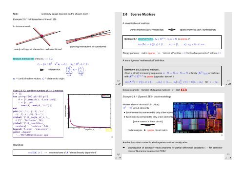
Example 2.6.1 (Sparse LSE in circuit modelling).
Modern electric circuits (VLSI chips):
10 5 − 10 7 circuit elements
• Each element is connected to only a few nodes
• Each node is connected to only a few elements
[In the case of a linear circuit]
nodal analysis ➤ sparse circuit matrix
✸
Heuristics:
Ôº½¿ ¾º
cond(A) ≫ 1 ↔ columns/rows of A “almost linearly dependent”
Another important context in which sparse matrices usually arise:
☛ discretization of boundary value problems for partial differential equations (→ 4th semester
course “Numerical treatment of PDEs”
Ôº½¼ ¾º