Numerical Methods Contents - SAM

✬
✩
Observations:
Theorem 4.2.7 (Convergence of CG method).
The iterates of the CG method for solving Ax = b (see Code 4.2.1) with A = A T s.p.d. satisfy
• CG much faster than gradient method (as expected, because it has “memory”)
• Both, CG and gradient method converge more slowly for larger sizes of Poisson matrices.
Convergence theory:
✸
∥
∥x − x (l)∥ ∥ ∥A ≤
≤ 2
( ) l
2 1 − √ 1
κ(A)
∥ ∥ ∥∥x
( ) 2l ( ) 2l − x
(0) ∥A
1 + √ 1 + 1 − √ 1
κ(A) κ(A)
(√ ) l κ(A) − 1
∥ ∥ ∥∥x
√ − x
(0) ∥A .
κ(A) + 1
A simple consequence of (4.1.2) and (4.2.1):
✫
(recall: κ(A) = spectral condition number of A, κ(A) = cond 2 (A))
✪
✬
Corollary 4.2.6 (“Optimality” of CG iterates).
Writing x ∗ ∈ R n for the exact solution of Ax = b the CG iterates satisfy
∥
∥x ∗ − x (l)∥ ∥ ∥A = min{‖y − x ∗ ‖ A : y ∈ x (0) + K l (A,r 0 )} , r 0 := b − Ax (0) .
✫
This paves the way for a quantitative convergence estimate:
✩
Ôº¿ º¾
✪
The estimate of this theorem √ confirms asymptotic linear convergence of the CG method (→
κ(A) − 1
Def. 3.1.4) with a rate of √
κ(A) + 1
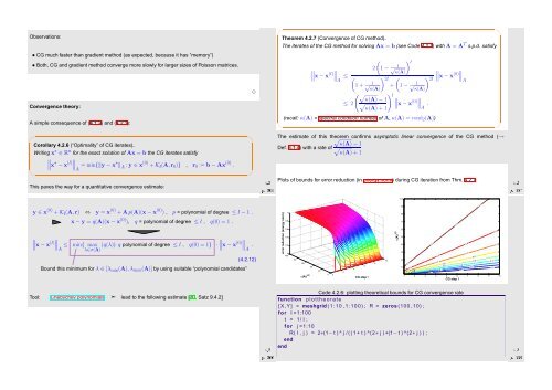
Plots of bounds for error reduction (in energy norm) during CG iteration from Thm. 4.2.7:
Ôº¿ º¾
100
y ∈ x (0) + K l (A,r) ⇔ y = x (0) + Ap(A)(x − x (0) ) , p = polynomial of degree ≤ l − 1 .
∥
∥x − x (l)∥ ∥ ∥A ≤
x − y = q(A)(x − x (0) ), q = polynomial of degree ≤ l , q(0) = 1 .
min{ max
λ∈σ(A) |q(λ)|: q polynomial of degree ≤ l , q(0) = 1} · ∥ ∥∥x − x
(0) ∥ ∥ ∥A .
Bound this minimum for λ ∈ [λ min (A), λ max (A)] by using suitable “polynomial candidates”
(4.2.12)
error reduction (energy norm)
1
0.8
0.6
0.4
0.2
0
100
80
60
κ(A) 1/2
40
20
0
0
2
4
6
CG step l
8
10
κ(A) 1/2
90
80
70
60
50
40
30
20
10
0.9
0.9
0.9
0.9
0.8 0.8 0.8 0.8
0.4 0.4 0.4
0.6 0.6 0.6
0.7 0.7 0.7 0.7
0.5 0.5 0.5
0.3 0.3 0.3
0.2
0.2 0.2 0.1
1 2 3 4 5 6 7 8 9 10
CG step l
Tool: Chebychev polynomials ➣ lead to the following estimate [20, Satz 9.4.2]
Code 4.2.6: plotting theoretical bounds for CG convergence rate
1 function p l o t t h e o r a t e
2 [ X, Y ] = meshgrid ( 1 : 1 0 , 1 : 1 0 0 ) ; R = zeros (100 ,10) ;
3 for I =1:100
4 t = 1 / I ;
5 for j =1:10
6 R( I , j ) = 2∗(1− t ) ^ j / ( ( 1 + t ) ^(2∗ j ) +(1− t ) ^(2∗ j ) ) ;
7 end
8 end
Ôº¿ º¾
Ôº¿ º¾
9