Numerical Methods Contents - SAM

More documents

Recommendations

Info

ootstrapping = use the same idea in a simpler version to get y(t 0 + c i h), noting that these values can be replaced by other approximations obtained by methods already constructed (this approach will be elucidated in the next example). 1 0.9 0.8 0.7 y(t) Explicit Euler Explicit trapezoidal rule Explicit midpoint rule 10 −1 s=1, Explicit Euler s=2, Explicit trapezoidal rule s=2, Explicit midpoint rule O(h 2 ) What error can we afford in the approximation of y(t 0 +c i h) (under the assumption that f is Lipschitz continuous)? y 0.6 0.5 0.4 0.3 error |y h (1)−y(1)| 10 −2 10 −3 0.2 10 −4 Goal: one-step error y(t 1 ) − y 1 = O(h p+1 ) 0.1 0 0 0.2 0.4 0.6 0.8 1 t Fig. 142 10 0 stepsize h 10 −2 10 −1 Fig. 143 This goal can already be achieved, if only y h (j/10), j = 1,...,10 for explicit RK-methods Errors at final time y h (1) − y(1) y(t 0 + c i h) is approximated up to an error O(h p ), because in (11.4.1) a factor of size h multiplies f(t 0 + c i ,y(t 0 + c i h)). Observation: obvious algebraic convergence with integer rates/orders explicit trapezoidal rule (11.4.3) order 2 explicit midpoint rule (11.4.4) order 2 This is accomplished by a less accurate discrete evolution than the one we are bidding for. Thus, we can construct discrete evolutions of higher and higher order, successively. Ôº½ ½½º Ôº¿ ½½º ✸ Example 11.4.1 (Construction of simple Runge-Kutta methods). The formulas that we have obtained follow a general pattern: Quadrature formula = trapezoidal rule (11.4.2): Q(f) = 1 2 (f(0) + f(1)) ↔ s = 2: c 1 = 0,c 2 = 1 , b 1 = b 2 = 1 2 , (11.4.2) and y(T) approximated by explicit Euler step (11.2.1) k 1 = f(t 0 ,y 0 ) , k 2 = f(t 0 + h,y 0 + hk 1 ) , y 1 = y 0 + h 2 (k 1 + k 2 ) . (11.4.3) (11.4.3) = explicit trapezoidal rule (for numerical integration of ODEs) Quadrature formula → simplest Gauss quadrature formula = midpoint rule (→ Ex. 10.2.1) & y( 1 2 (t 1+ t 0 )) approximated by explicit Euler step (11.2.1) Definition 11.4.1 (Explicit Runge-Kutta method). For b i ,a ij ∈ R, c i := ∑ i−1 j=1 a ij, i,j = 1, ...,s, s ∈ N, an s-stage explicit Runge-Kutta single step method (RK-SSM) for the IVP (11.1.5) is defined by ∑i−1 s∑ k i := f(t 0 + c i h,y 0 + h a ij k j ) , i = 1, ...,s , y 1 := y 0 + h b i k i . j=1 The k i ∈ R d are called increments. i=1 k 1 = f(t 0 ,y 0 ) , k 2 = f(t 0 + h 2 ,y 0 + h 2 k 1) , y 1 = y 0 + hk 2 . (11.4.4) (11.4.4) = explicit midpoint rule (for numerical integration of ODEs) ✸ Example 11.4.2 (Convergence of simple Runge-Kutta methods). IVP: ẏ = 10y(1 − y) (logistic ODE (11.1.1)), y(0) = 0.01, T = 1, Explicit single step methods, uniform timestep h. Ôº¾ ½½º Recall Rem. 11.2.4 to understand how the discrete evolution for an explicit Runge-Kutta method is specified in this definition by giving the formulas for the first step. This is a convention widely adopted in the literature about numerical methods for ODEs. Of course, the increments k i have to be computed anew in each timestep. Ôº ½½º
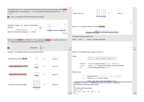
The implementation of an s-stage explicit Runge-Kutta single step method according to Def. 11.4.1 is straightforward: The increments k i ∈ R d are computed successively, starting from k 1 = f(t 0 + c 1 h,y 0 ). Only s f-evaluations and AXPY operations are required. • Kutta’s 3/8-rule: 0 0 0 0 0 1 1 3 3 0 0 0 2 3 −1 3 1 0 0 ➣ order = 4 1 1 −1 1 0 1 3 3 1 8 8 8 8 Shorthand notation for (explicit) Runge-Kutta methods Butcher scheme ✄ (Note: A is strictly lower triangular s × s-matrix) c A b T := . c 1 0 · · · 0 c 2 a 21 ... . . . ... . b 1 · · · b s c s a s1 · · · a s,s−1 0 (11.4.5) Remark 11.4.4 (“Butcher barriers” for explicit RK-SSM). order p 1 2 3 4 5 6 7 8 ≥ 9 minimal no.s of stages 1 2 3 4 6 7 9 11 ≥ p + 3 ✸ No general formula available so far Note that in Def. 11.4.1 the coefficients b i can be regarded as weights of a quadrature formula on [0, 1]: apply explicit Runge-Kutta single step method to “ODE” ẏ = f(t). Known: order p < number s of stages of RK-SSM Necessarily s∑ b i = 1 i=1 Ôº ½½º △ Ôº ½½º Example 11.4.3 (Butcher scheme for some explicit RK-SSM). Remark 11.4.5 (Explicit ODE integrator in MATLAB). • Explicit Euler method (11.2.1): 0 0 1 ➣ order = 1 Syntax: [t,y] = ode45(odefun,tspan,y0); • explicit trapezoidal rule (11.4.3): 0 0 0 1 1 0 1 2 1 2 ➣ order = 2 odefun : Handle to a function of type @(t,y) ↔ r.h.s. f(t,y) tspan : vector (t 0 , T) T , initial and final time for numerical integration y0 : (vector) passing initial state y 0 ∈ R d • explicit midpoint rule (11.4.4): 0 0 0 1 2 1 2 0 0 1 ➣ order = 2 Return values: t : temporal mesh {t 0 < t 1 < t 2 < · · · < t N−1 = t N = T } y : sequence (y k ) N k=0 (column vectors) • Classical 4th-order RK-SSM: 0 0 0 0 0 1 2 1 2 0 0 0 1 2 0 1 2 0 0 1 0 0 1 0 1 6 2 6 6 2 6 1 ➣ order = 4 Ôº ½½º Code 11.4.6: parts of MATLAB integrator ode45 1 function varargout = ode45 ( ode , tspan , y0 , options , v a r a r g i n ) 2 % Processing of input parameters omitted 3 % . 4 % Initialize method parameters. 5 pow = 1 / 5 ; 6 A = [ 1 / 5 , 3/10 , 4 /5 , 8 /9 , 1 , 1 ] ; 7 B = [ Ôº ½½º
Page 1 and 2:
2 Direct Methods for Linear Systems
Page 3 and 4:
III Integration of Ordinary Differe
Page 5 and 6:
Extra questions for course evaluati
Page 7 and 8:
1.1.2 Matrices Matrices = two-dimen
Page 9 and 10:
Remark 1.2.1 (Row-wise & column-wis
Page 11 and 12:
1.3 Complexity/computational effort
Page 13 and 14:
Syntax of BLAS calls: The functions
Page 15 and 16:
4 { 5 a ssert ( this−>n==B. n &&
Page 17 and 18:
34 long r t 0 ; 35 bool bStarted ;
Page 19 and 20:
Obviously, left multiplication with
Page 21 and 22:
❶: elimination step, ❷: backsub
Page 23 and 24:
A direct way to LU-decomposition:
Page 25 and 26:
Solution of LŨx = b: x ( ) 2ǫ = 1
Page 27 and 28:
numerically equivalent ˆ= same res
Page 29 and 30:
Code 2.4.8: Finding outeps in MATLA
Page 31 and 32:
Terminology: Def. 2.5.5 introduces
Page 33 and 34:
Example 2.5.5 (Instability of multi
Page 35 and 36:
Note: sensitivity gauge depends on
Page 37 and 38:
6 for i =1:20 7 n = 2^ i ; m = n /
Page 39 and 40:
0 20 40 60 80 100 120 140 160 180 2
Page 41 and 42:
Use sparse matrix format: 10 1 10 2
Page 43 and 44:
Envelope-aware LU-factorization: 0
Page 45 and 46:
0 20 40 60 80 100 0 20 0 20 0 20 De
Page 47 and 48:
Evident: symmetry of Ã − bbT a 1
Page 49 and 50:
9 ylabel ( ’ { \ b f c o n d i t
Page 51 and 52:
Mapping a ∈ K n to a multiple of
Page 53 and 54:
Then store G ij (a,b) as triple (i,
Page 55 and 56:
Recall: e i ˆ= i-th unit vector Ch
Page 57 and 58:
Computation of Choleskyfactorizatio
Page 59 and 60:
1 ∃ (partial) cyclic row permutat
Page 61 and 62:
Definition 3.1.3 (Local and global
Page 63 and 64:
Example 3.1.6 (quadratic convergenc
Page 65 and 66:
k |x (k) − π| L 1−L |x (k) −
Page 67 and 68:
(x (k) ) k∈N0 Cauchy sequence ➤
Page 69 and 70:
Termination criterion for contracti
Page 71 and 72:
Given x (k) ∈ I, next iterate :=
Page 73 and 74:
secant method ( MATLAB implementati
Page 75 and 76:
Assuming p = 1: p > 1: ∥ C ∥e (
Page 77 and 78:
This is a simple computation: DG(x)
Page 79 and 80:
k x (k) ǫ k := ‖x ∗ − x (k)
Page 81 and 82:
Code 3.4.14: Damped Newton method (
Page 83 and 84:
MATLAB-CODE: Broyden method (3.4.11
Page 85 and 86:
Algorithm 4.1.3 (Steepest descent).
Page 87 and 88:
Example 4.1.8 (Convergence of gradi
Page 89 and 90:
4.2.1 Krylov spaces Definition 4.2.
Page 91 and 92:
Remark 4.2.3 (A posteriori terminat
Page 93 and 94:
10 figure ; view ([ −45 ,28]) ; m
Page 95 and 96:
Idea: Solve Ax = b approximately in
Page 97 and 98:
eplaced with κ(A) ! 4.4.2 Iteratio
Page 99 and 100:
For circuit of Fig. 55 at angular f
Page 101 and 102:
(Linear) generalized eigenvalue pro
Page 103 and 104:
10 0 10 1 matrix size n d = eig(A)
Page 105 and 106:
0 50 100 150 200 250 300 350 400 45
Page 107 and 108:
1 2 3 k ρ (k) EV ρ (k) EW ρ (k)
Page 109 and 110:
✬ ✩ ✬ ✩ Lemma 5.3.4 (Ncut a
Page 111 and 112:
In other words, roundoff errors may
Page 113 and 114:
Theory: linear convergence of (5.3.
Page 115 and 116:
error in eigenvalue 10 0 10 −2 10
Page 117 and 118:
✬ Residuals r 0 ,...,r m−1 gene
Page 119 and 120:
Algebraic view of the Arnoldi proce
Page 121 and 122:
5.5 Singular Value Decomposition Re
Page 123 and 124:
Illustration: columns = ONB of Im(A
Page 125 and 126:
✬ Theorem 5.5.7 (best low rank ap
Page 127 and 128:
Reassuring: Remark 6.0.4 (Pseudoinv
Page 129 and 130:
Consider the linear least squares p
Page 131 and 132:
Goal: Euclidean distance of y ∈ R
Page 133 and 134:
6.5 Non-linear Least Squares If (6.
Page 135 and 136:
0 2 4 6 8 10 12 14 16 value of ∥
Page 137 and 138:
Definition 7.1.1 (Discrete convolut
Page 139 and 140:
Expand a 0 ,...,a n−1 and b 0 , .
Page 141 and 142:
(7.2.2) is a simple consequence of
Page 143 and 144:
Dominant coefficients of a signal a
Page 145 and 146:
11 c = f f t ( y ) ; 12 13 figure (
Page 147 and 148:
Two-dimensional trigonometric basis
Page 149 and 150:
8 end 9 t1 = min ( t1 , toc ) ; 10
Page 151 and 152:
Step II: for k =: rq + s, 0 ≤ r <
Page 153 and 154:
MATLAB-CODE Sine transform function
Page 155 and 156:
△ Example 7.5.2 (Linear regressio
Page 157 and 158:
[23, Ch. IX] presents the topic fro
Page 159 and 160:
Code 8.1.3: Horner scheme, polynomi
Page 161 and 162:
1.2 equality in (8.2.10) for y := (
Page 163 and 164:
ecursive definition: p i (t) ≡ y
Page 165 and 166: a 1 = y 1 − a 0 t 1 − t 0 = y 1
Page 167 and 168: Observations: Strong oscillations o
Page 169 and 170: −1 −0.8 −0.6 −0.4 −0.2 0
Page 171 and 172: 8.5.3 Chebychev interpolation: comp
Page 173 and 174: 9.1 Shape preserving interpolation
Page 175 and 176: 9.2.2 Piecewise polynomial interpol
Page 177 and 178: Interpolation of the function: f(x)
Page 179 and 180: 2 % Plot convergence of approximati
Page 181 and 182: 9.4 Splines Definition 9.4.1 (Splin
Page 183 and 184: ➤ Linear system of equations with
Page 185 and 186: y i+1 t i−1 t i t i+1 y i−1 y i
Page 187 and 188: 35 h= d i f f ( t ) ; 36 d e l t a
Page 189 and 190: 1 0.9 Function f 1 0.9 Function f
Page 191 and 192: f 10 Numerical Quadrature Numerical
Page 193 and 194: f • n = 1: Trapezoidal rule • n
Page 195 and 196: For fixed local n-point quadrature
Page 197 and 198: Equidistant trapezoidal rule (order
Page 199 and 200: Heuristics: A quadrature formula ha
Page 201 and 202: 20 Zeros of Legendre polynomials in
Page 203 and 204: |quadrature error| 10 0 Numerical q
Page 205 and 206: f f • line 9: estimate for global
Page 207 and 208: Model: autonomous Lotka-Volterra OD
Page 209 and 210: Example 11.1.6 (Transient circuit s
Page 211 and 212: y y 1 y(t) y 0 t t 0 t 1 Fig. 133 e
Page 213 and 214: for discrete evolution defined on I
Page 215: ⇒ if y ∈ C 2 ([0, T]), then y(t
Page 219 and 220: Example 11.5.2 (Blow-up). ✸ toler
Page 221 and 222: However, it would be foolish not to
Page 223 and 224: 0 0.2 0.4 0.6 0.8 1 1.2 1.4 1.6 1.8
Page 225 and 226: 4 3 2 abstol = 0.000010, reltol = 0
Page 227 and 228: ✸ ✸ Motivated by the considerat
Page 229 and 230: 0 1 2 3 4 5 6 u(t),v(t) 0.01 0.008
Page 231 and 232: MATLAB-CODE : Explicit integration
Page 233 and 234: Shorthand notation for Runge-Kutta
Page 235 and 236: 13 Structure Preservation 13.1 Diss
Page 237 and 238: [18] G. GOLUB AND C. VAN LOAN, Matr
Page 239 and 240: linear in Gauss-Newton method, 538
Page 241 and 242: Chebychev nodes, 678 double, 634 fo
Page 243 and 244: x∗ n y ˆ= discrete periodic conv
Page 245 and 246: Gaussian elimination with pivoting
show all

Numerical Methods Contents - SAM

You also want an ePaper? Increase the reach of your titles

Delete template?

Save as template?