Numerical Methods Contents - SAM

Idea: Partition integration domain [a,b] by mesh (grid, → Sect.9.2) M := {a =
x 0 < x 1 < ... < x m = b}
Apply quadrature formulas from Sects. 10.2, 10.4 on sub-intervals I j :=
[x j−1 , x j ], j = 1, ...,m, and sum up.
composite quadrature rule
Analogy: global polynomial interpolation ←→ piecewise polynomial interpolation
(→ Sect. 9.2)
Formulas (10.3.2), (10.3.3) directly suggest efficient implementation with minimal number of f-
evaluations.
✸
How to rate the “quality” of a composite quadrature formula ?
Note: Here we only consider one and the same quadrature formula (local quadrature formula) applied
on all sub-intervals.
Clear:
It is impossible to predict the quadrature error, unless the integrand is known.
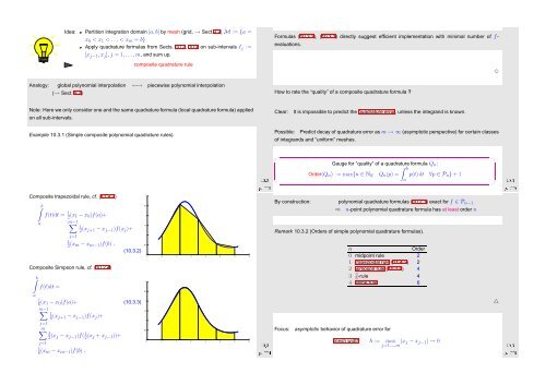
Example 10.3.1 (Simple composite polynomial quadrature rules).
Possible:
Predict decay of quadrature error as m → ∞ (asymptotic perspective) for certain classes
of integrands and “uniform” meshes.
✬
✩
Ôº¿ ½¼º¿
✫
Gauge for “quality” of a quadrature formula Q n :
∫ b
Order(Q n ) := max{n ∈ N 0 : Q n (p) = p(t) dt ∀p ∈ P n } + 1
a
Ôº ½¼º¿
✪
Composite trapezoidal rule, cf. (11.4.2)
∫b
a
f(t)dt = 1 2 (x 1 − x 0 )f(a)+
m−1 ∑
1
2 (x j+1 − x j−1 )f(x j )+
j=1
1
2 (x m − x m−1 )f(b) .
Composite Simpson rule, cf. (10.2.4)
∫b
f(t)dt =
a
1
6 (x 1 − x 0 )f(a)+
m−1 ∑
1
6 (x j+1 − x j−1 )f(x j )+
(10.3.2)
(10.3.3)
3
2.5
2
1.5
1
0.5
2.5
1.5
0
−1 0 1 2 3 4 5 6
3
2
By construction:
polynomial quadrature formulas (10.2.1) exact for f ∈ P n−1
⇒ n-point polynomial quadrature formula has at least order n
Remark 10.3.2 (Orders of simple polynomial quadrature formulas).
n
Order
0 midpoint rule 2
1 trapezoidal rule (11.4.2) 2
2 Simpson rule (10.2.4) 4
3 3 8 -rule 4
4 Milne rule 6
△
j=1
m∑
2
3 (x j − x j−1 )f( 2 1(x j + x j−1 ))+
j=1
1
6 (x m − x m−1 )f(b) .
1
0.5
0
−1 0 1 2 3 4 5 6
Ôº ½¼º¿
Focus:
asymptotic behavior of quadrature error for
mesh width h := max
j=1,...,m |x j − x j−1 | → 0
Ôº ½¼º¿