Numerical Methods Contents - SAM

Attention:
strong oscillations of the interpolation polynomials of high degree on uniformly spaced nodes!
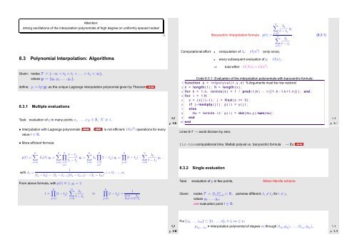
8.3 Polynomial Interpolation: Algorithms
✸
i=0
Barycentric interpolation formula p(t) = n∑
Computational effort: computation of λ i : O(n 2 ) (only once),
every subsequent evaluation of p:
⇒ total effort O(Nn) + O(n 2 )
n∑
i=0
O(n),
λ i
t − t i
y i
. (8.3.1)
λ i
t − t i
Given: nodes T := {−∞ < t 0 < t 1 < . .. < t n < ∞},
values y := {y 0 , y 1 ,...,y n },
define: p := I T (y) as the unique Lagrange interpolation polynomial given by Theorem 8.2.1.
8.3.1 Multiple evaluations
Task: evaluation of p in many points x 1 , ...,x N ∈ R, N ≫ 1.
• Interpolation with Lagrange polynomials (8.2.3) , (8.2.4) is not efficient: O(n 2 ) operations for every
value t ∈ R.
• More efficient formula:
p(t) =
with λ i =
n∑
L i (t) y i =
i=0
n∑
i=0
n∏
j=0
j≠i
t − t j
t i − t j
y i =
n∑ ∏ n n∏ n∑
λ i (t − t j ) y i = (t − t j ) ·
i=0
j=0
j≠i
1
(t i − t 0 ) · · · (t i − t i−1 )(t i − t i+1 ) · · · (t i − t n ) , i = 0,...,n.
From above formula, with p(t) ≡ 1, y i = 1:
1 =
n∏
(t − t j )
j=0
n∑
λ i
t − t
i=0 i
⇒
j=0
n∏
1
(t − t j ) = ∑ ni=0 λ i
j=0
t−t i
i=0
λ i
t − t i
y i .
Ôº º¿
Code 8.3.1: Evaluation of the interpolation polynomials with barycentric formula
1 function p = i n t p o l y v a l ( t , y , x ) % Arguments must be row vectors!
2 n = length ( t ) ; N = length ( x ) ;
3 for k = 1 : n , lambda ( k ) = 1 / prod ( t ( k ) − t ( [ 1 : k−1,k +1:n ] ) ) ; end ;
4 for i = 1 :N
5 z = ( x ( i )−t ) ; j = find ( z == 0) ;
6 i f (~ isempty ( j ) ) , p ( i ) = y ( j ) ;
7 else
Ôº º¿
8 mu = lambda . / z ; p ( i ) = dot (mu, y ) /sum(mu) ;
9 end
10 end
Lines 6-7 → avoid division by zero.
tic-toc-computational time, Matlab polyval vs. barycentric formula → Ex. 8.3.3.
8.3.2 Single evaluation
Task: evaluation of p in few points, Aitken-Neville scheme
Given: nodes T := {t j } n j=0 ⊂ R, pairwise different, t i ≠ t j for i ≠ j,
values y 0 , ...,y n ,
one evaluation point t ∈ R.
Ôº º¿
For {i 0 ,...,i m } ⊂ {0, . ..,n}, 0 ≤ m ≤ n:
p i0 ,...,i m = interpolation polynomial of degree m through (t i0 , y i0 ),...,(t im , y im ),
Ôº º¿