Numerical Methods Contents - SAM

Given x (k) ∈ I, next iterate := zero of model function: h(x (k+1) ) = 0, where
h(x) :=
a
x + b + c (rational function) such that F (j) (x (k) ) = h (j) (x (k) ) , j = 0, 1, 2 .
In the previous example Newton’s method performed rather poorly. Often its convergence can be
boosted by converting the non-linear equation to an equivalent one (that is, one with the same solutions)
for another function g, which is “closer to a linear function”:
a
x (k) + b + c = a
F(x(k) ) , −
(x (k) + b) 2 = F ′ (x (k) 2a
) ,
(x (k) + b) 3 = F ′′ (x (k) ) .
Halley’s iteration for F(x) =
x (k+1) = x (k) − F(x(k) )
F ′ (x (k) ) ·
1
.
1 − 1 F(x (k) )F ′′ (x (k) )
2 F ′ (x (k) ) 2
1
(x + 1) 2 + 1
(x + 0.1) 2 − 1 , x > 0 : and x(0) = 0
k x (k) F(x (k) ) x (k) − x (k−1) x (k) − x ∗
1 0.19865959351191 10.90706835180178 -0.19865959351191 -0.84754290138257
2 0.69096314049024 0.94813655914799 -0.49230354697833 -0.35523935440424
Ôº¾½ ¿º¿
3 1.02335017694603 0.03670912956750 -0.33238703645579 -0.02285231794846
4 1.04604398836483 0.00024757037430 -0.02269381141880 -0.00015850652965
5 1.04620248685303 0.00000001255745 -0.00015849848821 -0.00000000804145
Compare with Newton method (3.3.1) for the same problem:
k x (k) F(x (k) ) x (k) − x (k−1) x (k) − x ∗
1 0.04995004995005 44.38117504792020 -0.04995004995005 -0.99625244494443
2 0.12455117953073 19.62288236082625 -0.07460112958068 -0.92165131536375
3 0.23476467495811 8.57909346342925 -0.11021349542738 -0.81143781993637
4 0.39254785728080 3.63763326452917 -0.15778318232269 -0.65365463761368
5 0.60067545233191 1.42717892023773 -0.20812759505112 -0.44552704256257
6 0.82714994286833 0.46286007749125 -0.22647449053641 -0.21905255202615
7 0.99028203077844 0.09369191826377 -0.16313208791011 -0.05592046411604
8 1.04242438221432 0.00592723560279 -0.05214235143588 -0.00377811268016
9 1.04618505691071 0.00002723158211 -0.00376067469639 -0.00001743798377
10 1.04620249452271 0.00000000058056 -0.00001743761199 -0.00000000037178
Assume F ≈ ̂F , where ̂F is invertible with an inverse ̂F −1 that can be evaluated with little effort.
g(x) := ̂F −1 (F(x)) ≈ x .
Then apply Newton’s method to g(x), using the formula for the derivative of the inverse of a function
d
dy ( ̂F −1 )(y) =
1
̂F ′ ( ̂F −1 (y))
Example 3.3.5 (Adapted Newton method).
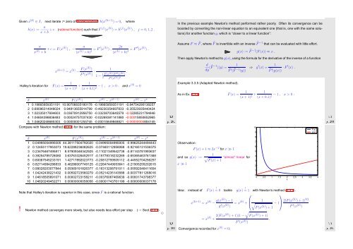
As in Ex. 3.3.4: F(x) =
Observation:
and so g(x) :=
x ≫ 1
F(x) + 1 ≈ 2x −2 for x ≫ 1
1
√
F(x) + 1
“almost” linear for
⇒ g ′ (x) =
1
̂F ′ (g(x)) · F ′ (x) .
1
(x + 1) 2 + 1
(x + 0.1) 2 − 1 , x > 0 :
10
9
8
7
6
5
4
3
2
1
F(x)
g(x)
0
0 0.5 1 1.5 2 2.5 3 3.5 4
x
Ôº¾¿ ¿º¿
Note that Halley’s iteration is superior in this case, since F is a rational function.
! Newton method converges more slowly, but also needs less effort per step (→ Sect. 3.3.3)
✸
Ôº¾¾ ¿º¿
Idea: instead of F(x) = ! 0 tackle g(x) = ! 1 with Newton’s method (3.3.1).
⎛
⎞
x (k+1) = x (k) − g(x(k) ) − 1
g ′ (x (k) = x (k) ⎜ 1 ⎟
+ ⎝√
− 1⎠ 2(F(x(k) ) + 1) 3/2
)
F(x (k) ) + 1 F ′ (x (k) )
√
= x (k) + 2(F(x(k) ) + 1)(1 − F(x (k) ) + 1)
F ′ (x (k) .
)
Convergence recorded for x (0) = 0:
Ôº¾ ¿º¿