Numerical Methods Contents - SAM

✬
Residuals r 0 ,...,r m−1 generated in CG iteration, Alg. 4.2.1 applied to Ax = z with x (0) = 0,
provide orthogonal basis for K m (A,z) (, if r k ≠ 0).
✫
✩
✪
Total computational effort for l steps of Lanczos process, if A has at most k non-zero entries per row:
O(nkl)
Inexpensive Ritz projection of Ax = λx onto K m (A,z):
orthogonal matrix
( )
VmAV T r0
m x = λx , V m :=
‖r 0 ‖ ,..., r m−1
∈ R n,m . (5.4.6)
‖r m−1 ‖
Note: Code 5.4.2 assumes that no residual vanishes. This could happen, if z 0 exactly belonged
to the span of a few eigenvectors. However, in practical computations inevitable round-off errors will
always ensure that the iterates do not stay in an invariant subspace of A, cf. Rem. 5.3.7.
recall: residuals generated by short recursions, see Alg. 4.2.1
✬
Lemma 5.4.1 (Tridiagonal Ritz projection from CG residuals).
V T mAV m is a tridiagonal matrix.
✫
✩
✪
Convergence (what we expect from the above considerations) → [13, Sect. 8.5])
In l-th step: λ n ≈ µ (l)
l , λ n−1 ≈ µ (l)
l−1 ,..., λ 1 ≈ µ (l)
1 ,
σ(T l ) = {µ (l)
1 , ...,µ(l) l }, µ (l)
1 ≤ µ (l)
2 ≤ · · · ≤ µ (l)
l .
Proof. Lemma 4.2.5: {r 0 ,...,r l−1 } is an orthogonal basis of K l (A,r 0 ), if all the residuals are nonzero.
As AK l−1 (A,r 0 ) ⊂ K l (A,r 0 ), we conclude the orthogonalityr T mAr j for all j = 0, ...,m−2.
Ôº º
the assertion of the theorem follows. ✷
Since
(V T mAV m
)
ij = rT i−1 Ar j−1 , 1 ≤ i,j ≤ m ,
⎛
⎞
α 1 β 1
β 1 α 2 β 2
β 2 α . 3
..
Vl H .
AV l =
.. . ..
=: T l ∈ K k,k [tridiagonal matrix]
...
⎜
⎟
⎝
... ... β k−1 ⎠
β k−1 α k
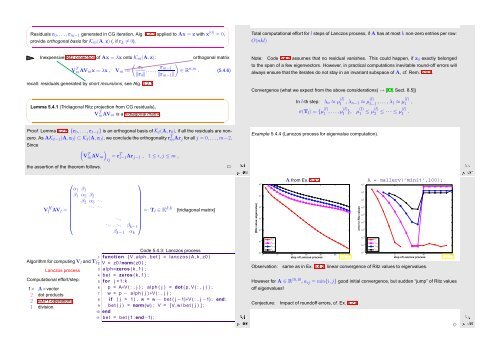
Example 5.4.4 (Lanczos process for eigenvalue computation).
A from Ex. 5.4.2
A = gallery(’minij’,100);
|Ritz value−eigenvalue|
10 2
10 1
10 0
10 0
10 −1
10 −2
error in Ritz values
10 −2
10 −4
10 −6
10 −8
Ôº º
10 2 step of Lanzcos process
10 4 step of Lanzcos process
Code 5.4.3: Lanczos process
1 function [ V, alph , bet ] = lanczos (A, k , z0 )
Algorithm for computingV l andT l :
2 V = z0 / norm( z0 ) ;
Lanczos process
3
4
alph=zeros ( k , 1 ) ;
bet = zeros ( k , 1 ) ;
Computational effort/step:
5 for j =1: k
1× A×vector
2 dot products
2 AXPY-operations
1 division
6 p = A∗V ( : , j ) ; alph ( j ) = dot ( p , V ( : , j ) ) ;
7 w = p − alph ( j ) ∗V ( : , j ) ;
8 i f ( j > 1) , w = w − bet ( j −1)∗V ( : , j −1) ; end ;
9 bet ( j ) = norm(w) ; V = [ V,w/ bet ( j ) ] ;
Ôº º
10 end
11 bet = bet ( 1 : end−1) ;
10 −3
10 −4
λ n
λ n−1
λ n−2
λ n−3
Fig. 77
0 5 10 15 20 25 30
Observation:
10 −10
10 −12
10 −14
λ n
λ n−1
λ n−2
λ n−3
Fig. 78
0 5 10 15
same as in Ex. 5.4.2, linear convergence of Ritz values to eigenvalues.
However for A ∈ R 10,10 , a ij = min{i,j} good initial convergence, but sudden “jump” of Ritz values
off eigenvalues!
Conjecture: Impact of roundoff errors, cf. Ex. 4.2.4
Ôº º
✸