Numerical Methods Contents - SAM

where
∫
|I| 2n+2 ∫
=
vol
I (n + 1)! (n) (C t,τ ) |f (n+1) (τ)| 2 dτdt ,
I } {{ }
≤2 (n−1)/2 /n!
Idea: choose nodes t 0 , ...,t n such that
‖w‖ L ∞ (I) is minimal!
Equivalent to finding q ∈ P n+1 , with leading coefficient = 1, such that ‖q‖ L ∞ (I) is
minimal.
Choice of t 0 , ...,t n = zeros of q (caution: t j must belong to I).
S n+1 := {x ∈ R n+1 : 0 ≤ x n ≤ x n−1 ≤ · · · ≤ x 1 ≤ 1} (unit simplex) ,
C t,τ := {x ∈ S n+1 : t 0 + x 1 (t 1 − t 0 ) + · · · + x n (t n − t n−1 ) + x n+1 (t − t n ) = τ} .
This gives the bound for the L 2 -norm of the error:
Notice:
⇒ ‖f − I T (f)‖ L 2 (I) ≤ 2(n−1)/4 |I| n+1 ( ∫
√ |f (n+1) (τ)| 2 1/2
dτ)
.
(n + 1)!n! I
(8.4.3)
∥
f ↦→ ∥f (n)∥ ∥ ∥L 2 (I) defines a seminorm on Cn+1 (I)
(Sobolev-seminorm, measure of the smoothness of a function).
△
Heuristic: • t ∗ extremal point of q ➙ |q(t ∗ )| = ‖q‖ L ∞ (I) ,
• q has n + 1 zeros in I,
• |q(−1)| = |q(1)| = ‖q‖ L ∞ (I) .
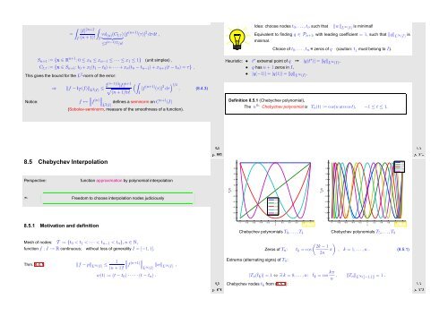
Definition 8.5.1 (Chebychev polynomial).
The n th Chebychev polynomial is T n (t) := cos(n arccost), −1 ≤ t ≤ 1.
Ôº º
Ôº½ º
8.5 Chebychev Interpolation
1
0.8
1
0.8
n=5
n=6
n=7
n=8
n=9
0.6
0.6
Perspective:
function approximation by polynomial interpolation
0.4
0.4
0.2
0.2
➣
✓
✒
Freedom to choose interpolation nodes judiciously
✏
✑
T n
(t)
0
−0.2
−0.4
n=0
n=1
T n
(t)
0
−0.2
−0.4
−0.6
n=2
−0.6
n=3
−0.8
n=4
−0.8
−1
−1
8.5.1 Motivation and definition
−1 −0.8 −0.6 −0.4 −0.2 0 0.2 0.4 0.6 0.8 1
−1 −0.8 −0.6 −0.4 −0.2 0 0.2 0.4 0.6 0.8 1
t
Fig. 102
t
Fig. 103
Chebychev polynomials T 0 ,...,T 4
Chebychev polynomials T 5 ,...,T 9
Mesh of nodes: T := {t 0 < t 1 < · · · < t n−1 < t n }, n ∈ N,
function f : I → R continuous; without loss of generality I = [−1, 1].
Thm. 8.4.1: ‖f − p‖ L ∞ (I) ≤ 1
∥
∥f (n+1)∥ ∥ ∥L
(n + 1)!
‖w‖ ∞ (I)
L ∞ (I) ,
w(t) := (t − t 0 ) · · · · · (t − t n ) .
Ôº¼ º
Zeros of T n :
Extrema (alternating signs) of T n :
( ) 2k − 1
t k = cos
2n π , k = 1, ...,n . (8.5.1)
|T n (t k )| = 1 ⇔ ∃ k = 0,...,n: t k = cos kπ n , ‖T n‖ L ∞ ([−1,1]) = 1 .
Chebychev nodes t k from (8.5.1):
Ôº¾ º