Numerical Methods Contents - SAM

0 20 40 60 80 100 120 140 160 180 200
0
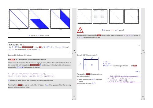
Sparse matrix
0
Sparse matrix: L factor
0
Sparse matrix: U factor
0
Pattern of A
0
0
Pattern of L
0
Pattern of U
20
20
20
2
2
2
2
40
40
40
4
4
4
4
60
60
60
80
80
80
6
6
6
6
100
100
100
8
8
8
8
120
120
120
10
10
10
10
140
160
140
160
140
160
12
12
0 2 4 6 8 10 12 0 2 4 6 8 10 12
nz = 31
nz = 121
Pattern of A −1 0 2 4 6 8 10 12
12
nz = 21
12
0 2 4 6 8 10 12
nz = 21
180
180
180
200
200
0 20 40 60 80 100 120 140 160 180 200
nz = 796
nz = 10299
200
0 20 40 60 80 100 120 140 160 180 200
nz = 10299
✸
!
L, U sparse ≠⇒ A −1 sparse !
A sparse ⇏ LU-factors sparse
Besides stability issues, see Ex. 2.5.3, this is another reason why using x = inv(A)*y instead of
y = A\b is usually a major blunder.
Definition 2.6.3 (Fill-in).
Let A = LU be an LU-factorization (→ Sect. 2.2) of A ∈ K n,n . If l ij ≠ 0 or u ij ≠ 0 though
a ij = 0, then we encounter fill-in at position (i,j).
Ôº½¿ ¾º
✸
Ôº½ ¾º
Example 2.6.13 (Sparse LU-factors).
Ex. 2.6.11 ➣ massive fill-in can occur for sparse matrices
This example demonstrates that fill-in can be largely avoided, if the matrix has favorable structure. In
this case a LSE with this particular system matrix A can be solved efficiently, that is, with a computational
effort O(nnz(A)) by Gaussian elimination.
Example 2.6.14 (“arrow matrix”).
⎛
α b T ⎞
A =
c D
⎜
⎟
⎝
⎠
,
α ∈ R ,
b,c ∈ R n−1 ,
D ∈ R n−1,n−1 regular diagonal matrix, → Def. 2.2.1
A = [diag(1:10),ones(10,1);ones(1,10),2];
[L,U] = lu(A); spy(A); spy(L); spy(U); spy(inv(A));
A is called an “arrow matrix”, see the pattern of non-zero entries below.
Recalling Rem. 2.2.7 it is easy to see that the LU-factors of A will be sparse and that their sparsity
patterns will be as depicted below.
Run algorithm 2.3.5 (Gaussian elimination
without pivoting):
factor matrices with O(n 2 ) non-zero
entries.
computational costs: O(n 3 )
(2.6.1)
Code 2.6.15: LU-factorization of arrow matrix
1 n = 10; A = [ n+1 , ( n: −1:1) ;
ones ( n , 1 ) , eye ( n , n ) ] ;
2 [ L ,U,P] = lu (A) ; spy ( L ) ; spy (U) ;
Ôº½ ¾º
Ôº½ ¾º