Numerical Methods Contents - SAM

∥
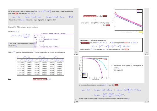
Let us abbreviate the error norm in step k by ǫ k := ∥x (k) − x ∗∥ ∥ ∥. In the case of linear convergence
(see Def. 3.1.4) assume (with 0 < L < 1)
10 0
x (0) = 0.4
x (0) = 0.6
x (0) = 1
ǫ k+1 ≈ Lǫ k ⇒ log ǫ k+1 ≈ log L + log ǫ k ⇒ log ǫ k+1 ≈ k log L + log ǫ 0 . (3.1.2)
We conclude that log L < 0 describes slope of graph in lin-log error chart.
△
Example 3.1.4 (Linearly convergent iteration).
Linear convergence as in Def. 3.1.4
⇕
error graphs = straight lines in lin-log scale
→ Rem. 3.1.3
iteration error
10 −1
10 −2
10 −3
Iteration (n = 1):
x (k+1) = x (k) + cos x(k) + 1
sinx (k) .
Code 3.1.5: simple fixed point iteration
1 y = [ ] ;
2 for i = 1:15
3 x = x + ( cos ( x ) +1) / sin ( x ) ;
4 y = [ y , x ] ;
5
x has to be initialized with the differentend
6 e r r = y − x ;
values for x 0 .
7 r a t e = e r r ( 2 : 1 5 ) . / e r r ( 1 : 1 4 ) ;
Note: x (15) replaces the exact solution x ∗ in the computation of the rate of convergence.
Ôº¾ ¿º½
Definition 3.1.7 (Order of convergence).
10 1 index of iterate
10 −4
1 2 3 4 5 6 7 8 9 10
A convergent sequence x (k) , k = 0, 1, 2, ..., in R n converges with order p to x ∗ ∈ R n , if
∥
∃C > 0: ∥x (k+1) − x ∗∥ ∥
∥ ∥∥x ≤ C (k) − x ∗∥ ∥p
∀k ∈ N 0 ,
and, in addition, C < 1 in the case p = 1 (linear convergence → Def. 3.1.4).
Fig. 31
✸
Ôº¾ ¿º½
k x (0) = 0.4 x (0) = 0.6 x (0) = 1
x (k) |x (k) −x (15) |
|x (k−1) −x (15) x (k) |x (k) −x (15) |
| |x (k−1) −x (15) x (k) |x (k) −x (15) |
| |x (k−1) −x (15) |
2 3.3887 0.1128 3.4727 0.4791 2.9873 0.4959
3 3.2645 0.4974 3.3056 0.4953 3.0646 0.4989
4 3.2030 0.4992 3.2234 0.4988 3.1031 0.4996
5 3.1723 0.4996 3.1825 0.4995 3.1224 0.4997
6 3.1569 0.4995 3.1620 0.4994 3.1320 0.4995
7 3.1493 0.4990 3.1518 0.4990 3.1368 0.4990
8 3.1454 0.4980 3.1467 0.4980 3.1392 0.4980
Rate of convergence ≈ 0.5
iteration error
10 −2
10 −4
10 −6
10 −8
10 −10
10 −12
p = 1.1
p = 1.2
10 −14 p = 1.4
p = 1.7
p = 2
10 −16
0 1 2 3 4 5 6 7 8 9 10 11
10 0 index k of iterates
✁
Qualitative error graphs for convergence of
order p
(lin-log scale)
Ôº¾ ¿º½
In the case of convergence of order p (p > 1) (see Def. 3.1.7):
ǫ k+1 ≈ Cǫ p k ⇒ log ǫ k+1 = log C + p log ǫ k ⇒ log ǫ k+1 = log C
⇒
log ǫ k+1 = − log C ( )
log C
p − 1 + p − 1 + log ǫ 0 p k+1 .
In this case, the error graph is a concave power curve (for sufficiently small ǫ 0 !)
k∑
p l + p k+1 log ǫ 0
l=0
Ôº¾ ¿º½