Numerical Methods Contents - SAM

0 0.2 0.4 0.6 0.8 1 1.2 1.4 1.6 1.8 2
0.05
0.045
Solving d t
y = a cos(y) 2 with a = 40.000000 by simple adaptive timestepping
Error vs. no. of timesteps for d t
y = a cos(y) 2 with a = 40.000000
10 1 no. N of timesteps
uniform timestep
adaptive timestep
Observations:
y
0.04
0.035
0.03
0.025
0.02
0.015
rtol = 0.400000
0.01
rtol = 0.200000
rtol = 0.100000
rtol = 0.050000
0.005
rtol = 0.025000
rtol = 0.012500
rtol = 0.006250
0
t
Fig. 150
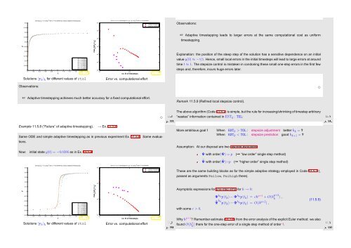
Solutions (y k ) k for different values of rtol
max k
|y(t k
)−y k
|
10 0
10 −1
10 −2
10 −3
10 −4
10 −5
10 1 10 2 10 3
Error vs. computational effort
Fig. 151
☞ Adaptive timestepping leads to larger errors at the same computational cost as uniform
timestepping.
Explanation: the position of the steep step of the solution has a sensitive dependence on an initial
value y(0) ≈ −π/2. Hence, small local errors in the initial timesteps will lead to large errors at around
time t ≈ 1. The stepsize control is mistaken in condoning these small one-step errors in the first few
steps and, therefore, incurs huge errors later.
Observations:
✸
☞ Adaptive timestepping achieves much better accuracy for a fixed computational effort.
Ôº ½½º
✸
Remark 11.5.9 (Refined local stepsize control).
The above algorithm (Code 11.5.2) is simple, but the rule for increasing/shrinking of timestep arbitrary
“wastes” information contained in EST k : TOL:
Ôº½ ½½º
Example 11.5.8 (“Failure” of adaptive timestepping). → Ex. 11.5.6
Same ODE and simple adaptive timestepping as in previous experiment Ex. 11.5.6. Same evaluations.
Now: initial state y(0) = −0.0386 as in Ex. 11.5.4
More ambitious goal ! When EST k > TOL : stepsize adjustment better h k = ?
When EST k < TOL : stepsize prediction good h k+1 = ?
Assumption: At our disposal are two discrete evolutions:
Ψ with order(Ψ) = p (➙ “low order” single step method)
˜Ψ with order(˜Ψ)>p (➙ “higher order” single step method)
Solving d t
y = a cos(y) 2 with a = 40.000000 by simple adaptive timestepping
Error vs. no. of timesteps for d t
y = a cos(y) 2 with a = 40.000000
0.05
0.04
0.03
uniform timestep
adaptive timestep
These are the same building blocks as for the simple adaptive strategy employed in Code 11.5.2 (,
passed as arguments Psilow, Psihigh there).
0.02
10 −1
y
0.01
0
−0.01
−0.02
−0.03
−0.04
rtol = 0.400000
rtol = 0.200000
rtol = 0.100000
rtol = 0.050000
rtol = 0.025000
rtol = 0.012500
rtol = 0.006250
−0.05
0 0.2 0.4 0.6 0.8 1 1.2 1.4 1.6 1.8 2
t
Fig. 152
Solutions (y k ) k for different values of rtol
max k
|y(t k
)−y k
|
10 0 no. N of timesteps
10 −2
10 −3
10 1 10 2 10 3
Error vs. computational effort
Fig. 153
Ôº¼ ½½º
Asymptotic expressions for one-step error for h → 0:
with some c > 0.
Ψ h ky(t k ) − Φ h ky(t k ) = ch p+1 + O(h p+2
k ) ,
˜Ψ hk y(t k ) − Φ h ky(t k ) = O(h p+2 ) ,
(11.5.5)
Ôº¾
Why h p+1 ? Remember estimate (11.3.6) from the error analysis of the explicit Euler method: we also
found O(h 2 k ) there for the one-step error of a single step method of order 1.
½½º