

Numerical Methods Contents - SAM
Numerical Methods Contents - SAM
Numerical Methods Contents - SAM

Create successful ePaper yourself
Turn your PDF publications into a flip-book with our unique Google optimized e-Paper software.
Consider discrete evolution of explicit Euler method (11.2.1) for ODE ẏ = My<br />
Ψ h y = y + hMy ↔ y k+1 = y k + hMy k .<br />
Perform the same transformation as above on the discrete evolution:<br />
1.5<br />
1<br />
0.5<br />
V −1 y k+1 = V −1 y k + hV −1 MV(V −1 y k )<br />
z k :=V −1 y k<br />
⇔<br />
(z k+1 ) i = (z k ) i + hλ i (z k )<br />
} {{ } i .<br />
ˆ= explicit Euler step for ż i = λ i z i<br />
(12.2.5)<br />
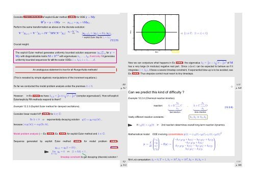
Im z<br />
0<br />
−0.5<br />
✁ {z ∈ C: |1 + z| < 1}<br />
Crucial insight:<br />
−1<br />
The explicit Euler method generates uniformly bounded solution sequences (y k ) ∞ k=0 for ẏ =<br />
My with diagonalizable matrix M ∈ R d,d with eigenvalues λ 1 , ...,λ d , if and only if it generates<br />
✗<br />
✖<br />
uniformly bounded sequences for all the scalar ODEs ż = λ i ż, i = 1,...,d.<br />
An analoguous statement is true for all Runge-Kutta methods!<br />
(This is revealed by simple algebraic manipulations of the increment equations.)<br />
So far we conducted the model problem analysis under the premises λ < 0.<br />
However: in Ex. 12.2.1 we have λ 1/2 = 1 2 α ±i √β − 1 4 α2 (complex eigenvalues!). How will explicit<br />
Euler/explicity RK-methods respond to them?<br />
Example 12.2.3 (Explicit Euler method for damped oscillations).<br />
Consider linear model IVP (12.1.1) for λ ∈ C:<br />
Re λ < 0 ⇒ exponentially decaying solution y(t) = y 0 exp(λt) ,<br />
because | exp(λt)| = exp(Re λt).<br />
✔<br />
✕<br />
Ôº½ ½¾º¾<br />
−1.5<br />
−2.5 −2 −1.5 −1 −0.5 0 0.5 1<br />
Re z<br />
Fig. 164<br />
Now we can conjecture what happens in Ex. 12.2.1: the eigenvalue λ 2 = 1 2 α − i √β − 1 4 α2 of M<br />
has a very large (in modulus) negative real part. Since ode45 can be expected to behave as if it<br />
integrates ż = λ 2 z, it faces a severe timestep constraint, if exponential blow-up is to be avoided, see<br />
Ex. 12.1.1. Thus stepsize control must resort to tiny timesteps.<br />
Can we predict this kind of difficulty ?<br />
Example 12.2.4 (Chemical reaction kinetics).<br />
reaction:<br />
k 2<br />
A + B<br />
←−<br />
−→ C<br />
k1<br />
} {{ }<br />
fast reaction<br />
k 4<br />
, A + C<br />
←−<br />
−→ D<br />
k3<br />
} {{ }<br />
slow reaction<br />
Vastly different reaction constants: k 1 ,k 2 ≫ k 3 , k 4<br />
If c A (0) > c B (0) ➢<br />
2nd reaction determines overall long-term reaction dynamics<br />
(12.2.6)<br />
Ôº½ ½¾º¾<br />
✸<br />
Model problem analysis (→ Ex. 12.1.1, Ex. 12.1.3) for explicit Euler method and λ ∈ C:<br />
Sequence generated by explicit Euler method (11.2.1) for model problem (12.1.1):<br />
y k+1 = y k (1 + hλ) . (12.1.2)<br />
lim y k = 0 ⇔ |1 + hλ| < 1 .<br />
k→∞<br />
timestep constraint to get decaying (discrete) solution !<br />
Ôº½ ½¾º¾<br />
Mathematical model: ODE involving concentrations y(t) = (c A (t), c B (t),c C (t), c D (t)) T<br />
⎛ ⎞ ⎛<br />
⎞<br />
c A<br />
−k 1 c A c B + k 2 c C − k 3 c A c C + k 4 c D<br />
ẏ := d ⎜c B<br />
⎟<br />
dt ⎝ cC ⎠ = f(y) := ⎜ −k 1 c A c B + k 2 c C<br />
⎟<br />
⎝ k 1 c A c B − k 2 c C − k 3 c A c C + k 4 c D<br />
⎠ .<br />
c D k 3 c A c C − k 4 c D<br />
MATLAB computation: t 0 = 0, T = 1, k 1 = 10 4 , k 2 = 10 3 , k 3 = 10, k 4 = 1<br />
Ôº¾¼ ½¾º¾


