Numerical Methods Contents - SAM

Proof.
(2.1.3) → induction w.r.t. n: After 1st step of elimination:
a (1)
ij = a ij − a i1
a 11
a 1j , i,j = 2,...,n ⇒ a (1)
ii > 0 .
Goal: Estimate relative perturbations in F(x) due to relative perturbations in x.
(cf. the same investigations for linear systems of equations in Sect. 2.5.5 and Thm. 2.5.9)
|a (1)
n ii | − ∑
|a (1) ∣
ij | = ∣∣aii
− a i1
j=2
j≠i
∣ ∣∣
∑ n ∣
a
a 1i − ∣a ij − a ∣
i1 ∣∣
a
11 a 1j
11
≥ a ii − |a i1||a 1i |
−
a 11
≥ a ii − |a i1||a 1i |
−
a 11
j=2
j≠i
n∑
j=2
j≠i
n∑
j=2
j≠i
|a ij | − |a i1|
a 11
∑ n |a 1j |
j=2
j≠i
|a ij | − |a i1 | a 11 − |a 1i |
a 11
≥ a ii −
n∑
|a ij | ≥ 0 .
j=1
j≠i
We assume that K n is equipped with some vector norm (→ Def. 2.5.1) and we use the induced
matrix norm (→ Def. 2.5.2) on K n,n .
Ax = y ⇒
∥
‖x‖ ≤ ∥A −1∥ ∥ ‖y‖
A(x + ∆x) = y + ∆y ⇒ A∆x = ∆y ⇒ ‖∆y‖ ≤ ‖A‖ ‖∆x‖
⇒
‖∆y‖
‖y‖ ≤ ‖A‖ ‖∆x‖
∥
∥A −1∥ ∥ −1 ‖x‖ = cond(A)‖∆x‖ ‖x‖ . (2.8.1)
relative perturbation in result
relative perturbation in data
A regular, diagonally dominant ⇒ partial pivoting according to (2.3.4) selects i-th row in i-th step.
➣
Condition number cond(A) (→ Def. 2.5.11) bounds amplification of relative error in argument
vector in matrix×vector-multiplication x ↦→ Ax.
△
Remark 2.7.4 (Telling MATLAB about matrix properties).
MATLAB-\ assumes generic matrix, cannot detect special properties of (fully populated) matrix (e.g.
Ôº½ ¾º
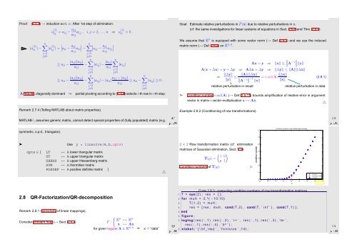
Example 2.8.2 (Conditioning of row transformations).
Ôº½½ ¾º
symmetrc, s.p.d., triangular).
Condition numbers of row transformation matrices
10 7 µ
10 6
➤ Use y = linsolve(A,b,opts)
opts ∈ { LT ↔ A lower triangular matrix
UT ↔ A upper triangular matrix
UHESS ↔ A upper Hessenberg matrix
SYM ↔ A Hermitian matrix
POSDEF ↔ A positive definite matrix }
△
2 × 2 Row transformation matrix (cf. elimination
matrices of Gaussian elimination, Sect. 2.2):
( )
1 0
T(µ) =
µ 1
Condition numbers of T(µ)
✄
condition number
10 5
10 4
10 3
10 2
10 1
10 0
2−norm
maximum norm
1−norm
10 −4 10 −3 10 −2 10 −1 10 0 10 1 10 2 10 3 10 4
Fig. 20
2.8 QR-Factorization/QR-decomposition
Remark 2.8.1 (Sensitivity of linear mappings).
{
K
Consider problem map (→ Sect. 2.5.2) F :
n ↦→ K n
x ↦→ Ax
Code 2.8.3: computing condition numbers of row transoformation matrices
1 T = eye ( 2 ) ; res = [ ] ;
2 for mult = 2.^( −10:10)
3 T ( 1 , 2 ) = mult ;
4 res = [ res ; mult , cond ( T , 2 ) , cond ( T , ’ i n f ’ ) , cond ( T , 1 ) ] ;
5 end
6 figure ;
7 loglog ( res ( : , 1 ) , res ( : , 2 ) , ’ r + ’ , res ( : , 1 ) , res ( : , 3 ) , ’m∗ ’ ,
res ( : , 1 ) , res ( : , 4 ) , ’ b^ ’ ) ;
Ôº½¼ ¾º
Ôº½¾ ¾º
for given regular A ∈ K n,n ➣ x ˆ= “data” 8 xlabel ( ’ { \ b f \mu} ’ , ’ f o n t s i z e ’ ,14) ;