Numerical Methods Contents - SAM

4.1 Descent Methods
2
16
16
1.5
14
14
12
Focus: Linear system of equations Ax = b, A ∈ R n,n , b ∈ R n , n ∈ N given,
1
12
10
with symmetric positive definite (s.p.d., → Def. 2.7.1) system matrix A
x 2
0.5
0
10
8
J(x 1
,x 2
)
8
6
➨ A-inner product (x,y) ↦→ x T Ay ⇒ “A-geometry”
−0.5
6
4
2
−1
4
0
Definition 4.1.1 (Energy norm).
A s.p.d. matrix A ∈ R n,n induces an energy norm
‖x‖ A := (x T Ax) 1/2 , x ∈ R n .
−1.5
0
−2
−2 −1.5 −1 −0.5 0 0.5 1 1.5 2
x 1
Fig. 41
2
−2
−2
0
x1
2 −2 −1.5 −1 −0.5 0 0.5 1 1.5 2
x 2
Fig. 42
Remark 4.1.1 (Krylov methods for complex s.p.d. system matrices).
✗
✖
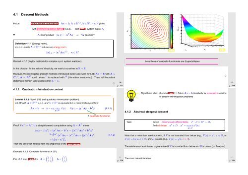
Level lines of quadratic functionals are (hyper)ellipses
✔
✕
In this chapter, for the sake of simplicity, we restrict ourselves to K = R.
However, the (conjugate) gradient methods introduced below also work for LSE Ax = b with A ∈
C n,n , A = A H s.p.d. when T is replaced with H (Hermitian transposed). Then, all theoretical
statements remain valid unaltered for K = C.
4.1.1 Quadratic minimization context
✬
Lemma 4.1.2 (S.p.d. LSE and quadratic minimization problem).
A LSE with A ∈ R n,n s.p.d. and b ∈ R n is equivalent to a minimization problem:
△
✩
Ôº¿¿¿ º½
Algorithmic idea: (Lemma 4.1.2 ➣) Solve Ax = b iteratively by successive solution
of simpler minimization problems
✸
Ôº¿¿ º½
✫
Ax = b ⇔
x = arg min
y∈R n J(y) , J(y) := 1 2 yT Ay − b T y . (4.1.1)
✪
4.1.2 Abstract steepest descent
A quadratic functional
Proof. If x ∗ := A −1 b a straightforward computation using A = A T shows
J(x) − J(x ∗ ) = 1 2 xT Ax − b T x − 1 2 (x∗ ) T Ax ∗ + b T x ∗
Then the assertion follows from the properties of the energy norm.
Example 4.1.2 (Quadratic functional in 2D).
Plot of J from (4.1.1) for A =
b=Ax ∗
= 1 2 xT Ax − (x ∗ ) T Ax + 1 2 (x∗ ) T Ax ∗
= 1 2 ‖x − x∗ ‖ 2 A . (4.1.2)
( ) (
2 1 1
, b =
1 2 1)
Ôº¿¿ º½
.
Task: Given continuously differentiable F : D ⊂ R n ↦→ R,
find minimizer x ∗ ∈ D: x ∗ = argmin F(x)
x∈D
Note that a minimizer need not exist, if F is not bounded from below (e.g., F(x) = x 3 , x ∈ R, or
F(x) = log x, x > 0), or if D is open (e.g., F(x) = √ x, x > 0).
The existence of a minimizer is guaranteed if F is bounded from below and D is closed (→ Analysis).
The most natural iteration:
Ôº¿¿ º½