Numerical Methods Contents - SAM

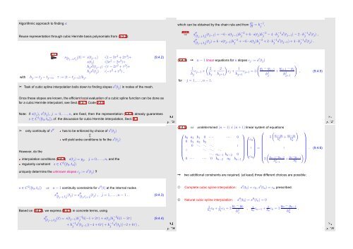
Algorithmic approach to finding s:
Reuse representation through cubic Hermite basis polynomials from (9.3.2):
which can be obtained by the chain rule and from dτ
dt = h−1 j
.
(9.4.4)
⇒ s ′′
|[t j−1 ,t j ] (t j−1) = −6 · s(t j−1 )h −2
j
s ′′
|[t j−1 ,t j ] (t j) = 6 · s(t j−1 )h −2
j
+ 6 · s(t j )h −2
j − 4 · h −1
j s ′ (t j−1 ) − 2 · h −1
j s ′ (t j ) ,
+ −6 · s(t j )h −2
j + 2 · h −1
j s ′ (t j−1 ) + 4 · h −1
j s ′ (t j ) .
(9.3.1)
with h j := t j − t j−1 , τ := (t − t j−1 )/h j .
s |[tj−1 ,t j ] (t) = s(t j−1) ·(1 − 3τ 2 + 2τ 3 )+
s(t j ) ·(3τ 2 − 2τ 3 )+
h j s ′ (t j−1 ) ·(τ − 2τ 2 + τ 3 )+
h j s ′ (t j ) ·(−τ 2 + τ 3 ) ,
➣ Task of cubic spline interpolation boils down to finding slopes s ′ (t j ) in nodes of the mesh.
(9.4.2)
(9.4.3) ➙ n − 1 linear equations for n slopes c j := s ′ (t j )
(
1 2
c
h j−1 + + 2 )
(
c
j h j h j + 1 yj − y j−1
c
j+1 h j+1 = 3
j+1 h 2 j
for j = 1,...,n − 1.
+ y )
j+1 − y j
h 2 , (9.4.5)
j+1
Once these slopes are known, the efficient local evaluation of a cubic spline function can be done as
for a cubic Hermite interpolant, see Sect. 9.3.1, Code 9.3.0.
Note: if s(t j ), s ′ (t j ), j = 0, ...,n, are fixed, then the representation (9.4.2) already guarantees
s ∈ C 1 ([t 0 ,t n ]), cf. the discussion for cubic Hermite interpolation, Sect. 9.3.
Ôº¾ º
Ôº¾ º
➣ only continuity of s ′′ has to be enforced by choice of s ′ (t j )
⇕
will yield extra conditions to fix the s ′ (t j )
However, do the
interpolation conditions (9.4.1) s(t j ) = y j , j = 0, ...,n, and the
regularity constraint s ∈ C 2 ([t 0 , t n ])
(9.4.5) ⇔ undetermined (n − 1) × (n + 1) linear system of equations
⎛
⎛
⎞
b 0 a 1 b 1 0 · · · · · · 0 ⎛ ⎞
0 b 1 a 2 b 2
c 3
0
0 ... . .. ... .
⎜ . . .. ... ...
⎜ .
⎟
⎟⎝
⎠ = .
⎝
... a n−1 b n−2 0 ⎠ ⎜
c
0 · · · · · · 0 b n−2 a 0 b n ⎝
n−1 3
(
y 1 −y 0
h 2 + y 2−y 1
1 h 2 2
)
(
y n−1 −y n−2
h 2 + y n−y n−1
n−1
h 2 n
⎞
. (9.4.6)
) ⎟
⎠
uniquely determine the unknown slopes c j := s ′ (t j ) ?
➙
two additional constraints are required, (at least) three different choices are possible:
s ∈ C 2 ([t 0 ,t n ]) ⇒ n − 1 continuity constraints for s ′′ (t) at the internal nodes
s ′′
|[t j−1 ,t j ] (t j) = s ′′
|[t j ,t j+1 ] (t j) , j = 1, ...,n − 1 . (9.4.3)
➀ Complete cubic spline interpolation: s ′ (t 0 ) = c 0 , s ′ (t n ) = c n prescribed.
➁ Natural cubic spline interpolation: s ′′ (t 0 ) = s ′′ (t n ) = 0
Based on (9.4.2), we express (9.4.3) in concrete terms, using
s ′′
|[t j−1 ,t j ] (t) = s(t j−1)h −2
j 6(−1 + 2τ) + s(t j )h −2
j 6(1 − 2τ)
+ h −1
j s ′ (t j−1 )(−4 + 6τ) + h −1
j s ′ (t j )(−2 + 6τ) ,
(9.4.4)
Ôº¾ º
2
h c 1 0 + h 1 c 1 1 = 3 y 1 − y 0
h 2 1
, 1
hn
c n−1 + h 2 c n n = 3 y n − y n−1
h 2 .
n
Ôº¾ º