

Numerical Methods Contents - SAM
Numerical Methods Contents - SAM
Numerical Methods Contents - SAM

You also want an ePaper? Increase the reach of your titles
YUMPU automatically turns print PDFs into web optimized ePapers that Google loves.
✬<br />
✩<br />
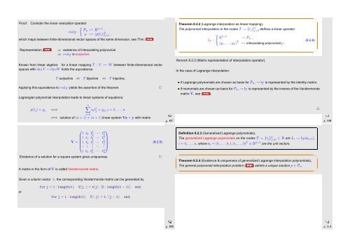
Proof.<br />
Consider the linear evaluation operator<br />
{<br />
Pn ↦→ R<br />
eval T :<br />
n+1 ,<br />
p ↦→ (p(t i )) n i=0 ,<br />
which maps between finite-dimensional vector spaces of the same dimension, see Thm. 8.1.1.<br />
Theorem 8.2.2 (Lagrange interpolation as linear mapping).<br />
The polynomial interpolation in the nodes T := {t j } n j=0 defines a linear operator<br />
{<br />
K n+1 → P n ,<br />
I T :<br />
(y 0 ,...,y n ) T ↦→ interpolating polynomial p .<br />
(8.2.6)<br />
Representation (8.2.4)<br />
⇒ existence of interpolating polynomial<br />
⇒ eval T is surjective<br />
✫<br />
✪<br />
Known from linear algebra: for a linear mapping T : V ↦→ W between finite-dimensional vector<br />
spaces with dimV = dimW holds the equivalence<br />
Remark 8.2.2 (Matrix representation of interpolation operator).<br />
In the case of Lagrange interpolation:<br />
T surjective ⇔ T bijective ⇔ T injective.<br />
Applying this equivalence to eval T yields the assertion of the theorem<br />
Lagrangian polynomial interpolation leads to linear systems of equations:<br />
✷<br />
• if Lagrange polynomials are chosen as basis for P n , → I T is represented by the identity matrix;<br />
• if monomials are chosen as basis for P n , → I T is represented by the inverse of the Vandermonde<br />
matrix V, see (8.2.5).<br />
p(t j ) = y j<br />
n∑<br />
⇐⇒<br />
a i t i j = y j, j = 0,...,n<br />
i=0<br />
⇐⇒ solution of (n + 1) × (n + 1) linear system Va = y with matrix<br />
Ôº¿ º¾<br />
△<br />
Ôº¿ º¾<br />
⎛<br />
1 t 0 t 2 0 · · · ⎞<br />
tn 0<br />
1 t 1 t 2 1<br />
V =<br />
· · · tn 1<br />
⎜1 t 2 t 2 2<br />
⎝<br />
· · · tn 2⎟<br />
. . . . .. . ⎠ . (8.2.5)<br />
1 t n t 2 n · · · t n Existence of a solution for a square system gives uniqueness.<br />
✷<br />
A matrix in the form of V is called Vandermonde matrix.<br />
Definition 8.2.3 (Generalized Lagrange polynomials).<br />
The generalized Lagrange polynomials on the nodes T = {t j } n j=0 ⊂ R are L i := I T (e i+1 ),<br />
i = 0,...,n, where e i = (0,...,0, 1, 0,...,0) T ∈ R n+1 are the unit vectors.<br />
✬<br />
Theorem 8.2.4 (Existence & uniqueness of generalized Lagrange interpolation polynomials).<br />
The general polynomial interpolation problem (8.2.2) admits a unique solution p ∈ P n .<br />
✫<br />
✩<br />
✪<br />
Given a column vector t, the corresponding Vandermonde matrix can be generated by<br />
or<br />
for j = 1 : length(t); V(j, :) = t(j).ˆ[0 : length(t −1)]; end;<br />
for j = 1 : length(t); V(:,j) = t.ˆ(j −1); end;<br />
Ôº¿ º¾<br />
Ôº¼ º¾


