Numerical Methods Contents - SAM

This is a simple computation:
DG(x) = ADF(x) ⇒ DG(x) −1 G(x) = DF(x) −1 A −1 AF(x) = DF(x) −1 F(x) .
Use affine invariance as guideline for
• convergence theory for Newton’s method: assumptions and results should be affine invariant, too.
• modifying and extending Newton’s method: resulting schemes should preserve affine invariance.
Remark 3.4.5 (Simplified Newton method).
Simplified Newton Method: use the same DF(x (k) ) for more steps
➣ (usually) merely linear convergence instead of quadratic convergence
Remark 3.4.6 (Numerical Differentiation for computation of Jacobian).
△
△
Remark 3.4.4 (Differentiation rules).
→ Repetition: basic analysis
Statement of the Newton iteration (3.4.1) for F : R n ↦→ R n given as analytic expression entails
computing the Jacobian DF . To avoid cumbersome component-oriented considerations, it is useful
to know the rules of multidimensional differentiation:
Let V , W be finite dimensional vector spaces, F : D ⊂ V ↦→ W sufficiently smooth. The differential
DF(x) of F in x ∈ V is the unique
linear mapping DF(x) : V ↦→ W ,
such that ‖F(x + h) − F(x) − DF(h)h‖ = o(‖h‖) ∀h, ‖h‖ < δ .
• For F : V ↦→ W linear, i.e. F(x) = Ax, A matrix ➤ DF(x) = A.
• Chain rule: F : V ↦→ W , G : W ↦→ U sufficiently smooth
D(G ◦ F)(x)h = DG(F(x))(DF(x))h , h ∈ V , x ∈ D . (3.4.2)
• Product rule: F : D ⊂ V ↦→ W , G : D ⊂ V ↦→ U sufficiently smooth, b : W × U ↦→ Z bilinear
T(x) = b(F(x), G(x)) ⇒ DT(x)h = b(DF(x)h,G(x)) + b(F(x), DG(x)h) ,
h ∈ V ,x ∈ D .
△
(3.4.3)
Ôº¿¼ ¿º
If DF(x) is not available
(e.g. when F(x) is given only as a procedure):
Numerical Differentiation:
Caution: impact of roundoff errors for small h !
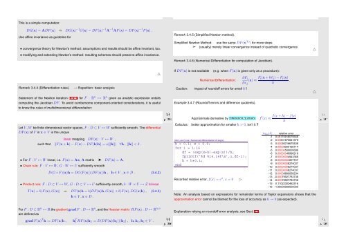
Example 3.4.7 (Roundoff errors and difference quotients).
Approximate derivative by difference quotient:
Calculus: better approximation for smaller h > 0, isn’t it ?
MATLAB-CODE: Numerical differentiation of exp(x)
h = 0.1; x = 0.0;
for i = 1:16
df = (exp(x+h)-exp(x))/h;
fprintf(’%d %16.14f\n’,i,df-1);
h = h*0.1;
end
Recorded relative error, f(x) = e x , x = 0
✄
∂F i
(x) ≈ F i(x + h⃗e j ) − F i (x)
.
∂x j h
f ′ (x) ≈
f(x + h) − f(x)
h
log 10 (h) relative error
-1 0.05170918075648
-2 0.00501670841679
-3 0.00050016670838
-4 0.00005000166714
-5 0.00000500000696
-6 0.00000049996218
-7 0.00000004943368
-8 -0.00000000607747
-9 0.00000008274037
-10 0.00000008274037
-11 0.00000008274037
-12 0.00008890058234
-13 -0.00079927783736
-14 -0.00079927783736
-15 0.11022302462516
-16 -1.00000000000000
△
Ôº¿¼ ¿º
.
Note: An analysis based on expressions for remainder terms of Taylor expansions shows that the
approximation error cannot be blamed for the loss of accuracy as h → 0 (as expected).
For F : D ⊂ R n ↦→ R the gradientgradF : D ↦→ R n , and the Hessian matrix HF(x) : D ↦→ R n,n
Ôº¿¼ ¿º
are defined as
gradF(x) T h := DF(x)h , h T 1 HF(x)h 2 := D(DF(x)(h 1 ))(h 2 ) , h,h 1 ,h 2 ∈ V .
Explanation relying on roundoff error analysis, see Sect. 2.4:
Ôº¿¼ ¿º