Numerical Methods Contents - SAM

Advantages:
• “foolproof”
• requires only F evaluations
Example 3.3.3 (Newton method in 1D). (→ Ex. 3.2.1)
Drawbacks:
Merely linear( convergence: ) |x (k) − x ∗ | ≤ 2 −k |b − a|
|b − a|
log 2 steps necessary
tol
Remark 3.3.2. MATLAB function fzero is based on bisection approach.
△
Newton iterations for two different scalar non-linear equation with the same solution sets:
F(x) = xe x − 1 ⇒ F ′ (x) = e x (1 + x) ⇒ x (k+1) = x (k) − x(k) e x(k) − 1
e x(k) (1 + x (k) ) = (x(k) ) 2 + e −x(k)
1 + x (k)
F(x) = x − e −x ⇒ F ′ (x) = 1 + e −x ⇒ x (k+1) = x (k) − x(k) − e −x(k)
= 1 + x(k)
1 + e −x(k) 1 + e x(k)
Ex. 3.2.1 shows quadratic convergence ! (→ Def. 3.1.7)
✸
3.3.2 Model function methods
ˆ= class of iterative methods for finding zeroes of F :
Idea: Given: approximate zeroes x (k) , x (k−1) , ...,x (k−m)
➊ replace F with model function ˜F
(using function values/derivative values in x (k) , x (k−1) ,...,x (k−m) )
➋ x (k+1) := zero of ˜F
(has to be readily available ↔ analytic formula)
Distinguish (see (3.1.1)):
Ôº¾ ¿º¿
Newton iteration (3.3.1)
Φ(x) = x − F(x)
F ′ (x)
From Lemma 3.2.7:
⇒
ˆ= fixed point iteration (→ Sect.3.2) with iteration function
Φ ′ (x) = F(x)F ′′ (x)
(F ′ (x)) 2 ⇒ Φ ′ (x ∗ ) = 0 , , if F(x ∗ ) = 0, F ′ (x ∗ ) ≠ 0 .
Newton method locally quadratically convergent (→ Def. 3.1.7) to zero x ∗ , if F ′ (x ∗ ) ≠ 0
3.3.2.2 Special one-point methods
Ôº¾ ¿º¿
one-point methods : x (k+1) = Φ F (x (k) ), k ∈ N (e.g., fixed point iteration → Sect. 3.2)
multi-point methods : x (k+1) = Φ F (x (k) , x (k−1) , . ..,x (k−m) ), k ∈ N, m = 2, 3,....
Idea underlying other one-point methods:
non-linear local approximation
Useful, if a priori knowledge about the structure of F (e.g. about F being a rational function, see
3.3.2.1 Newton method in scalar case
below) is available. This is often the case, because many problems of 1D zero finding are posed for
functions given in analytic form with a few parameters.
Assume:
F : I ↦→ R continuously differentiable
Prerequisite: Smoothness of F : F ∈ C m (I) for some m > 1
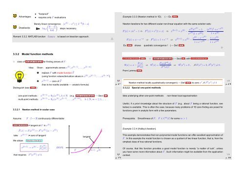
model function:= tangent at F in x (k) :
˜F(x) := F(x (k) ) + F ′ (x (k) )(x − x (k) )
Example 3.3.4 (Halley’s iteration).
take
We obtain
x (k+1) := zero of tangent
Newton iteration
tangent
This example demonstrates that non-polynomial model functions can offer excellent approximation of
F . In this example the model function is chosen as a quotient of two linear function, that is, from the
simplest class of true rational functions.
x (k+1) := x (k) − F(x(k) )
F ′ (x (k) )
that requires F ′ (x (k) ) ≠ 0.
, (3.3.1)
F
x (k+1)
x (k)
Ôº¾ ¿º¿
Of course, that this function provides a good model function is merely “a matter of luck”, unless
you have some more information about F . Such information might be available from the application
context.
Ôº¾¼ ¿º¿