Numerical Methods Contents - SAM

✬
Theorem 10.4.1 (Existence of n-point quadrature formulas of order 2n).
Let { ¯Pn
}n∈N 0
be a family of non-zero polynomials that satisfies
• ¯P n ∈ P n ,
∫ 1
• q(t) ¯P n (t) dt = 0 for all q ∈ P n−1 (L 2 (] − 1, 1[)-orthogonality),
−1
• The set {ξj n}m j=1 , m ≤ n, of real zeros of ¯P n is contained in [−1, 1].
Then
✫
Q n (f) :=
m∑
ωj n f(ξn j )
j=1
with weights chosen according to Rem. 10.3.11 provides a quadrature formula of order 2n on
[−1, 1].
✩
✪
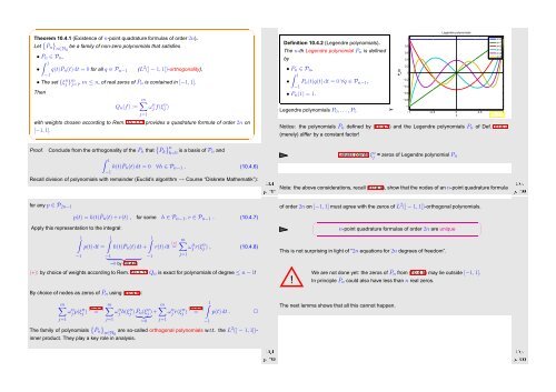
Definition 10.4.2 (Legendre polynomials).
The n-th Legendre polynomial P n is defined
by
• P n ∈ P n ,
∫ 1
• P n (t)q(t) dt = 0 ∀q ∈ P n−1 ,
−1
• P n (1) = 1.
−1
Legendre polynomials P 0 , . ..,P 5 ➣
−1 −0.5 0 0.5 1
P n
(t)
1
0.8
0.6
0.4
0.2
0
−0.2
−0.4
−0.6
−0.8
Legendre polynomials
t
n=0
n=1
n=2
n=3
n=4
n=5
Fig. 114
Notice: the polynomials ¯P n defined by (10.4.5) and the Legendre polynomials P n of Def. 10.4.2
(merely) differ by a constant factor!
Proof. Conclude from the orthogonality of the ¯P { } n
n that ¯P k k=0 is a basis of P n and
∫ 1
h(t) ¯P n (t) dt = 0 ∀h ∈ P n−1 . (10.4.6)
−1
Recall division of polynomials with remainder (Euclid’s algorithm → Course “Diskrete Mathematik”):
Ôº ½¼º
Gauss points ξ n j = zeros of Legendre polynomial P n
Note: the above considerations, recall (10.4.4), show that the nodes of an n-point quadrature formula
Ôº ½¼º
for any p ∈ P 2n−1
p(t) = h(t) ¯P n (t) + r(t) , for some h ∈ P n−1 , r ∈ P n−1 . (10.4.7)
of order 2n on [−1, 1] must agree with the zeros of L 2 (] − 1, 1[)-orthogonal polynomials.
Apply this representation to the integral:
∫1 ∫1
p(t) dt = h(t) ¯P n (t) dt
−1
−1
} {{ }
=0 by (10.4.6)
∫1
+
−1
r(t) dt (∗) =
m∑
ωj n r(ξn j ) , (10.4.8)
j=1
✗
✖
n-point quadrature formulas of order 2n are unique
This is not surprising in light of “2n equations for 2n degrees of freedom”.
✔
✕
(∗): by choice of weights according to Rem. 10.3.11 Q n is exact for polynomials of degree ≤ n − 1!
!
We are not done yet: the zeros of ¯P n from (10.4.5) may lie outside [−1, 1].
In principle ¯P n could also have less than n real zeros.
By choice of nodes as zeros of ¯P n using (10.4.6):
m∑
j=1
ωj n p(ξn j ) (10.4.7)
=
m∑
ωj n h(ξn j ) ¯P
m∑
n (ξj n } {{ }
) +
j=1 =0 j=1
ωj n r(ξn j ) (10.4.8)
=
∫1
−1
p(t) dt .
✷
The next lemma shows that all this cannot happen.
The family of polynomials { ¯P n
}n∈N 0
are so-called orthogonal polynomials w.r.t. the L 2 (] − 1, 1[)-
inner product. They play a key role in analysis.
Ôº ½¼º
Ôº¼¼ ½¼º