

Numerical Methods Contents - SAM
Numerical Methods Contents - SAM
Numerical Methods Contents - SAM

You also want an ePaper? Increase the reach of your titles
YUMPU automatically turns print PDFs into web optimized ePapers that Google loves.
Reassuring:<br />
Remark 6.0.4 (Pseudoinverse).<br />
stable (→ Def.2.5.5) implementation (for dense matrices).<br />
This means: if ‖r‖ 2 ≪ 1 ➤ condition of the least squares problem ≈ cond 2 (A)<br />
if ‖r‖ 2 “large” ➤ condition of the least squares problem ≈ cond 2 2 (A)<br />
△<br />
By Lemma 6.0.1 the solution operator of the least squares problem (6.0.3) defines a linear mapping<br />
b ↦→ x, which has a matrix representation.<br />
Definition 6.0.2 (Pseudoinverse). The pseudoinverse A + ∈ K n,m of A ∈ K m,n is the matrix<br />
representation of the (linear) solution operator R m ↦→ R n , b ↦→ x of the least squares problem<br />
(6.0.3) ‖Ax − b‖ → min, ‖x‖ → min.<br />
6.1 Normal Equations<br />
Setting: A ∈ R m,n , m ≥ n, with full rank rank(A) = n.<br />
MATLAB:<br />
P = pinv(A) computes the pseudoinverse.<br />
△<br />
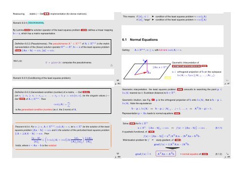
b<br />
{Ax,x ∈ R n }<br />
Geometric interpretation of<br />
linear least squares problem (6.0.3):<br />
Remark 6.0.5 (Conditioning of the least squares problem).<br />
Ôº¼ º¼<br />
Ax<br />
Fig. 89<br />
x ˆ= orthogonal projection of b on the subspace<br />
Im(A) := Span { (A) :,1 ,...,(A) :,n<br />
}<br />
.<br />
Ôº¼ º½<br />
Definition 6.0.3 (Generalized condition (number) of a matrix, → Def. 2.5.11).<br />
Let σ 1 ≥ σ 2 ≥ σ r > σ r+1 = . .. = σ p = 0, p := min{m, n}, be the singular values (→<br />
Def. 5.5.2) of A ∈ K m,n . Then<br />
cond 2 (A) := σ 1<br />
σ r<br />
is the generalized condition (number) (w.r.t. the 2-norm) of A.<br />
Geometric interpretation: the least squares problem (6.0.3) amounts to searching the point p ∈<br />
Im(A) nearest (w.r.t. Euclidean distance) to b ∈ R m .<br />
Geometric intuition, see Fig. 89: p is the orthogonal projection of b onto Im(A), that is b − p ⊥<br />
Im(A). Note the equivalence<br />
b − p ⊥ Im(A) ⇔ b − p ⊥ (A) :,j , j = 1, ...,n ⇔ A H (b − p) = 0 ,<br />
Representation p = Ax leads to normal equations (6.1.2).<br />
✬<br />
Theorem 6.0.4. For m ≥ n, A ∈ K m,n , rank(A) = n, let x ∈ K n be the solution of the least<br />
squares problem ‖Ax − b‖ → min and ̂x the solution of the perturbed least squares problem<br />
‖(A + ∆A)̂x − b‖ → min. Then<br />
(<br />
)<br />
‖x − ̂x‖ · 2 ≤ 2 cond<br />
‖x‖ 2 (A) + cond 2 2 (A) ‖r‖ 2 ‖∆A‖2<br />
2 ‖A‖ 2 ‖x‖ 2 ‖A‖ 2<br />
✫<br />
holds, where r = Ax − b is the residual.<br />
✩<br />
Ôº¼ º¼<br />
✪<br />
Solve (6.0.3) for b ∈ R m<br />
x ∈ R n : ‖Ax − b‖ 2 → min ⇔ f(x) := ‖Ax − b‖ 2 2 → min . (6.1.1)<br />
A quadratic functional, cf. (4.1.1)<br />
f(x) = ‖Ax − b‖ 2 2 = xH (A H A)x − 2b H Ax + b H b .<br />
Minimization problem for f ➣ study gradient, cf. (4.1.4)<br />
Ôº¼ º½<br />
gradf(x) = ! 0: A H Ax = A H b = normal equation of (6.1.1) (6.1.2)<br />
gradf(x) = 2(A H A)x − 2A H b .


