Numerical Methods Contents - SAM

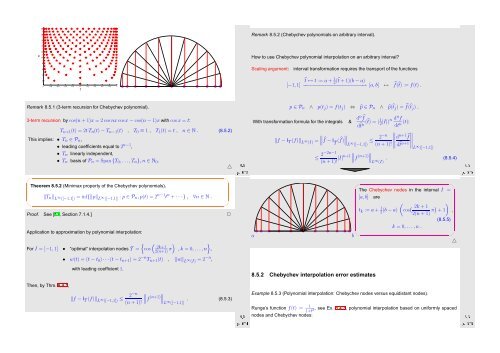
−1 −0.8 −0.6 −0.4 −0.2 0 0.2 0.4 0.6 0.8 1
20
18
Remark 8.5.2 (Chebychev polynomials on arbitrary interval).
16
14
n
12
10
How to use Chebychev polynomial interpolation on an arbitrary interval?
8
6
Scaling argument:
interval transformation requires the transport of the functions
4
2
t
[−1, 1]
̂t ↦→ t := a + 1 2 (̂t + 1)(b − a)
−−−−−−−−−−−−−−−−−−−−−→ [a,b] ↔ ̂f(̂t) := f(t) .
Remark 8.5.1 (3-term recursion for Chebychev polynomial).
p ∈ P n ∧ p(t j ) = f(t j ) ⇔ ̂p ∈ P n ∧ ̂p(̂t j ) = ̂f(̂t j ) .
3-term recursion by cos(n + 1)x = 2 cos nx cosx − cos(n − 1)x with cos x = t:
T n+1 (t) = 2tT n (t) − T n−1 (t) , T 0 ≡ 1 , T 1 (t) = t , n ∈ N . (8.5.2)
This implies: • T n ∈ P n ,
• leading coefficients equal to 2 n−1 ,
• T n linearly independent,
• T n basis of P n = Span {T 0 ,...,T n }, n ∈ N 0 .
△
Ôº¿ º
dn ̂f
With transformation formula for the integrals &
d̂t n (̂t) = ( 1 2 |I|)n dn f
dt n (t):
∥
∥ ∥∥
‖f − I T (f)‖ L ∞ (I) = ̂f − ÎT
( ̂f)
∥ ≤ 2−n
dn+1 ̂f ∥∥∥∥L L ∞ ([−1,1]) (n + 1)! ∥ d̂t n+1 ∞ ([−1,1])
≤ 2−2n−1
(n + 1)! |I|n+1 ∥ ∥ ∥f
(n+1) ∥ ∥ ∥L ∞ (I) . (8.5.4)
Ôº º
✬
✩
Theorem 8.5.2 (Minimax property of the Chebychev polynomials).
✫
‖T n ‖ L ∞ ([−1,1]) = inf{‖p‖ L ∞ ([−1,1]) : p ∈ P n,p(t) = 2 n−1 t n + · · · } , ∀n ∈ N .
Proof. See [13, Section 7.1.4.] ✷
Application to approximation by polynomial interpolation:
{ ( ) }
For I = [−1, 1] • “optimal” interpolation nodes T = cos 2k+1
2(n+1) π , k = 0, ...,n ,
• w(t) = (t − t 0 ) · · · (t − t n+1 ) = 2 −n T n+1 (t) , ‖w‖ L ∞ (I) = 2−n ,
✪
a
b
✬
The Chebychev nodes in the interval I =
[a,b] are
(
t k := a + 1 2 (b − a) cos ( )
2k + 1
2(n + 1) π) + 1 ,
✫
k = 0,...,n .
(8.5.5)
✩
✪
△
with leading coefficient 1.
8.5.2 Chebychev interpolation error estimates
Then, by Thm. 8.4.1,
‖f − I T (f)‖ L ∞ ([−1,1]) ≤
2−n
∥
∥f (n+1)∥ ∥ ∥L
(n + 1)!
. ∞ ([−1,1]) (8.5.3)
Ôº º
Example 8.5.3 (Polynomial interpolation: Chebychev nodes versus equidistant nodes).
Runge’s function f(t) = 1
1+t2, see Ex. 8.4.3, polynomial interpolation based on uniformly spaced
nodes and Chebychev nodes:
Ôº º