Numerical Methods Contents - SAM

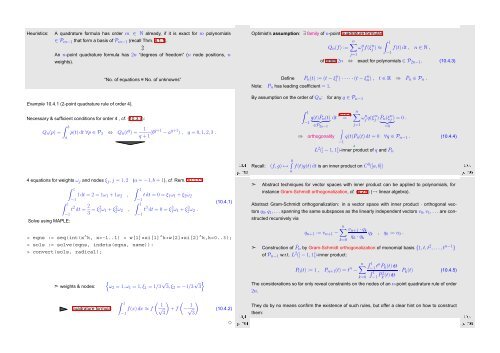
Heuristics:
A quadrature formula has order m ∈ N already, if it is exact for m polynomials
∈ P m−1 that form a basis of P m−1 (recall Thm. 8.1.1).
⇕
An n-point quadrature formula has 2n “degrees of freedom” (n node positions, n
weights).
Optimist’s assumption: ∃ family of n-point quadrature formulas
n∑
∫ 1
Q n (f) := ωj n f(ξn j ) ≈ f(t) dt , n ∈ N ,
j=1
−1
of order 2n ⇔ exact for polynomials ∈ P 2n−1 . (10.4.3)
“No. of equations = No. of unknowns”
Define ¯Pn (t) := (t − ξ n 1 ) · · · · · (t − ξn n) , t ∈ R ⇒ ¯P n ∈ P n .
Note: ¯P n has leading coefficient = 1.
Example 10.4.1 (2-point quadrature rule of order 4).
By assumption on the order of Q n :
for any q ∈ P n−1
Necessary & sufficient conditions for order 4 , cf. (10.3.7):
∫ b
Q n (p) = p(t) dt ∀p ∈ P 3 ⇔ Q n (t q ) = 1
a
q + 1 (bq+1 − a q+1 ) , q = 0, 1, 2, 3 .
∫ 1
n∑
q(t) ¯P n (t) dt (10.4.3)
= ω
−1 } {{ }
j n q(ξn j ) ¯P n (ξj n ) = 0 .
} {{ }
∈P 2n−1 j=1 =0
∫1
⇒ orthogonality q(t) ¯P n (t) dt = 0 ∀q ∈ P n−1 . (10.4.4)
−1
Ôº¿ ½¼º
Recall:
L 2 (] − 1, 1[)-inner product of q and ¯P n
∫b
(f, g) ↦→ f(t)g(t) dt is an inner product on C 0 ([a,b])
a
Ôº ½¼º
4 equations for weights ω j and nodes ξ j , j = 1, 2 (a = −1,b = 1), cf. Rem. 10.3.11
∫ 1
∫ 1
1 dt = 2 = 1ω 1 + 1ω 2 , t dt = 0 = ξ 1 ω 1 + ξ 2 ω 2
−1
−1
∫ 1
t 2 dt = 2 ∫ 1
−1 3 = ξ2 1 ω 1 + ξ2 2 ω 2 , t 3 dt = 0 = ξ1 3 ω 1 + ξ2 3 ω 2 .
−1
Solve using MAPLE:
(10.4.1)
> eqns := seq(int(x^k, x=-1..1) = w[1]*xi[1]^k+w[2]*xi[2]^k,k=0..3);
> sols := solve(eqns, indets(eqns, name)):
> convert(sols, radical);
➣
Abstract techniques for vector spaces with inner product can be applied to polynomials, for
instance Gram-Schmidt orthogonalization, cf. (4.2.6) (→ linear algebra).
Abstract Gram-Schmidt orthogonalization: in a vector space with inner product · orthogonal vectors
q 0 , q 1 , ... spanning the same subspaces as the linearly independent vectors v 0 , v 1 , ... are constructed
recursively via
q n+1 := v n+1 −
n∑
k=0
v n+1 · q k
q k · q k
q k , q 0 := v 0 .
➣ Construction of ¯P n by Gram-Schmidt orthogonalization of monomial basis {1, t,t 2 , ...,t n−1 }
of P n−1 w.r.t. L 2 (] − 1, 1[)-inner product:
➣ weights & nodes:
{
ω 2 = 1,ω 1 = 1,ξ 1 = 1/3 √ 3,ξ 2 = −1/3 √ }
3
¯P 0 (t) := 1 ,
¯Pn+1 (t) = t n −
n∑
k=0
∫ 1−1
t n ¯P k (t)dt
∫ 1−1 ¯P 2
k (t)dt · ¯P k (t) (10.4.5)
The considerations so far only reveal constraints on the nodes of an n-point quadrature rule of order
2n.
quadrature formula:
∫ 1
−1
( ) 1
f(x) dx ≈ f √3 + f
(−√ 1 )
3
(10.4.2)
Ôº ½¼º
✸
They do by no means confirm the existence of such rules, but offer a clear hint on how to construct
them:
Ôº ½¼º