Numerical Methods Contents - SAM

where k ∈ R s ˆ= denotes the vector (k 1 , ...,k s ) T /λ of increments, and z := λh.
y 1 = S(z)y 0 with S(z) := 1 + zb T (I − zA) −1 1 = det(I − zA + z1b T ) . (12.1.7)
The first formula for S(z) immediately follows from (12.1.6), the second is a consequence of
Cramer’s rule.
Remark 12.1.4 (Stepsize control detects instability).
Always look at the bright side of life:
Ex. 12.0.1, 12.1.2: Stepsize control guarantees acceptable solutions, with a hefty price tag however.
△
Thus we have proved the following theorem.
✬
Theorem 12.1.1 (Stability function of explicit Runge-Kutta methods).
The discrete evolution Ψ h λ
of an explicit s-stage Runge-Kutta single step method (→ Def. 11.4.1)
✩
12.2 Stiff problems
with Butcher scheme c A bT (see (11.4.5)) for the ODE ẏ = λy is a multiplication operator
according to
Ψ h λ = 1 + zbT (I − zA) −1 1 = det(I − zA + z1b
} {{ }
T ) , z := λh , 1 = (1, ...,1) T ∈ R s .
stability function S(z)
✫
½¾º½
✪
Thm. 12.1.1 ⇒ S ∈ P s
Ôº¼
Objection: The IVP (12.1.1) may be an oddity rather than a model problem: the weakness of explicit
Runge-Kutta methods discussed in the previous section may be just a peculiar response to an unusual
situation.
This section will reveal that the behavior observed in Ex. 12.0.1 and Ex. 12.1.1 is typical for a large
class of problems and that the model problem (12.1.1) really represents a “generic case”.
Ôº½½ ½¾º¾
Remember from Ex. 12.1.3: for sequence (|y k |) ∞ k=0 produced by explicit Runge-Kutta method applied
to IVP (12.1.1) holds y k = S(λh) k y 0 .
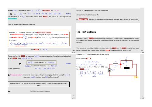
Example 12.2.1 (Transient simulation of RLC-circuit).
Circuit from Ex. 11.1.6
✄
C
(|y k |) ∞ k=0 non-increasing ⇔ |S(λh)| ≤ 1 ,
(12.1.8)
(|y k |) ∞ k=0 exponentially increasing ⇔ |S(λh)| > 1 .
On the other hand: ∀S ∈ P s : lim
|z|→∞ |S(z)| = ∞
timestep constraint: In order to avoid exponentially increasing (qualitatively wrong for λ < 0)
sequences (y k ) ∞ k=0 we must have |λh| sufficiently small.
ü + α ˙u + βu = g(t) ,
α := (RC) −1 , β = (LC) −1 , g(t) = α ˙U s .
Transformation to linear 1st-order ODE, see
Rem. 11.1.7, v := ˙u
( ( ( ) ( )
˙u˙v)
0 1 u 0
=
− .
−β −α)
v g(t)
}{{} } {{ }
=:ẏ
=:f(t,y)
U s (t)
R
u(t)
L
Fig. 161
Small timesteps may have to be used for stability reasons, though accuracy may not require
them!
Inefficient numerical integration
Ôº½¼ ½¾º½
Ôº½¾ ½¾º¾