Numerical Methods Contents - SAM

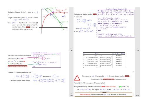
Illustration of idea of Newton’s method for n = 2:
✄
Sought: intersection point x ∗ of the curves
F 1 (x) = 0 and F 2 (x) = 0.
Idea: x (k+1) = the intersection of two straight
lines (= zero sets of the components of the
model function, cf. Ex. 2.5.11) that are approximations
of the original curves
x 2
F 2 (x) = 0
˜F 1
x ∗ (x) = 0
F 1 (x) = 0
x (k+1) x (k)
˜F 2 (x) = 0
x 1
Code 3.4.2: Newton iteration in 2D
1 F = @( x ) [ x ( 1 )^2−x ( 2 ) ^4; x ( 1 )−x ( 2 ) ^3 ] ;
2 DF = @( x ) [2∗ x ( 1 ) , −4∗x ( 2 ) ^3; 1 , −3∗x ( 2 ) ^ 2 ] ;
Realization of Newton iteration (3.4.1): 3 x = [ 0 . 7 ; 0 . 7 ] ; x_ast = [ 1 ; 1 ] ; t o l = 1E−10;
4
1. Solve LSE
(
2x1 −4x 3 )
5 res = [ 0 , x ’ , norm( x−x_ast ) ] ;
1 −3x 2 ∆x (k) 6 s = feval (DF, x ) \ feval ( F , x ) ; x = x−s ;
=
7 2
res = [ res ; 1 ,x ’ , norm( x−x_ast ) ] ; k =2;
(
x 2
− 1 − x 4 )
8 while (norm( s ) > t o l ∗norm( x ) )
2
x 1 − x 3 9,
s = DF( x ) \ F ( x ) ; x = x−s ;
2
where x (k) = (x 1 , x 2 ) T 10 res = [ res ; k , x ’ , norm( x−x_ast ) ] ;
.
11 k = k +1;
2. Set x (k+1) = x (k) + ∆x (k) 12 end
13
14 l o g d i f f = d i f f ( log ( res ( : , 4 ) ) ) ;
15 r a t e s = l o g d i f f ( 2 : end ) . / l o g d i f f ( 1 : end−1) ;
Ôº¿¼½ ¿º
Ôº¿¼¿ ¿º
MATLAB template for Newton method:
Solve linear system:
A\b = A −1 b → Chapter 2
F,DF: function handles
A posteriori termination criterion
MATLAB-CODE: Newton’s method
function x = newton(x,F,DF,tol)
for i=1:MAXIT
s = DF(x) \ F(x);
x = x-s;
if (norm(s) < tol*norm(x))
return; end;
end
k x (k) ǫ k := ‖x ∗ − x (k) ‖ 2
0 (0.7, 0.7) T 4.24e-01
1 (0.87850000000000, 1.064285714285714) T 1.37e-01
2 (1.01815943274188, 1.00914882463936) T 2.03e-02
3 (1.00023355916300, 1.00015913936075) T 2.83e-04
4 (1.00000000583852, 1.00000002726552) T 2.79e-08
5 (0.999999999999998, 1.000000000000000) T 2.11e-15
6 (1, 1) T ✸
Example 3.4.1 (Newton method in 2D).
(
x 2
F(x) = 1 − x 4 )
2
x 1 − x 3 , x =
2
( x1
x 2
)
Jacobian (analytic computation): DF(x) =
(
∈ R 2 1
with solution F
1)
(
∂x1 F 1 (x) ∂ x2 F 1 (x)
∂ x1 F 2 (x) ∂ x2 F 2 (x)
= 0 .
) (
2x1 −4x
= 3 1 −3x 2 2
)
!
New aspect for n ≫ 1 (compared to n = 1-dimensional case, section. 3.3.2.1):
Computation of the Newton correction is eventually costly!
Remark 3.4.3 (Affine invariance of Newton method).
Ôº¿¼¾ ¿º
An important property of the Newton iteration (3.4.1): affine invariance → [11, Sect .1.2.2]
set G(x) := AF(x) with regular A ∈ R n,n so that F(x ∗ ) = 0 ⇔ G(x ∗ ) = 0 .
✗
✖
affine invariance: Newton iteration for G(x) = 0 is the same for all regular A !
✔
✕
Ôº¿¼ ¿º