

Numerical Methods Contents - SAM
Numerical Methods Contents - SAM
Numerical Methods Contents - SAM

You also want an ePaper? Increase the reach of your titles
YUMPU automatically turns print PDFs into web optimized ePapers that Google loves.
9 ylabel ( ’ { \ b f c o n d i t i o n number } ’ , ’ f o n t s i z e ’ ,14) ;<br />
10 t i t l e ( ’ Condition numbers o f row t r a n s f o r m a t i o n matrices ’ ) ;<br />
11 legend ( ’2−norm ’ , ’maximum norm ’ , ’1−norm ’ , ’ l o c a t i o n ’ , ’ southeast ’ ) ;<br />
12 p r i n t −depsc2 ’ . . / PICTURES/ rowtrfcond . eps ’ ;<br />
all rows/columns are pairwise orthogonal (w.r.t. Euclidean inner product),<br />
| detQ| = 1, and all eigenvalues ∈ {z ∈ C: |z| = 1}.<br />
‖QA‖ 2 = ‖A‖ 2 for any matrix A ∈ K n,m<br />
Observation: cond(T(µ)) large for large µ<br />
As explained in Sect. 2.2, Gaussian (forward) elimination can be viewed as successive multiplication<br />
with elimination matrices. If an elimination matrix has a large condition number, then small relative errors<br />
in the entries of intermediate matrices caused by earlier roundoff errors can experience massive<br />
amplification and, thus, spoil all further steps (➤ loss of numerical stability, Def. 2.5.5).<br />
Drawbacks of LU-factorization:<br />
often pivoting required (➞ destroys structure, Ex. 2.6.21, leads to fill-in)<br />
Possible (theoretical) instability of partial pivoting → Ex. 2.5.2<br />
Therefore, the entries of elimination matrices should be kept small, and this is the main rationale<br />
behind (partial) pivoting (→ Sect. 2.3), which ensures that multipliers have modulus ≤ 1 throughout<br />
forward elimination.<br />
Ôº½¿ ¾º<br />
✸<br />
Stability problems of Gaussian elimination without pivoting are due to the fact that row transformations<br />
can convert well-conditioned matrices to ill-conditioned matrices, cf. Ex. 2.5.2<br />
Which bijective row transformations preserve the Euclidean condition number of a matrix ?<br />
Ôº½ ¾º<br />
➣ transformations hat preserve the Euclidean norm of a vector !<br />
Recall from linear algebra:<br />
Investigate algorithms that use orthogonal/unitary row transformations to convert a matrix to<br />
upper triangular form.<br />
Definition 2.8.1 (Unitary and orthogonal matrices).<br />
• Q ∈ K n,n , n ∈ N, is unitary, if Q −1 = Q H .<br />
• Q ∈ R n,n , n ∈ N, is orthogonal, if Q −1 = Q T .<br />
✬<br />
Theorem 2.8.2 (Criteria for Unitarity).<br />
✩<br />
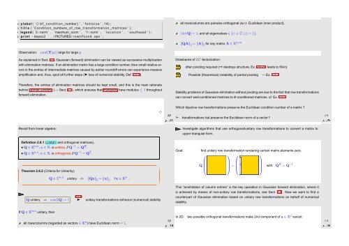
Goal:<br />
find unitary row transformation rendering certain matrix elements zero.<br />
⎛ ⎞ ⎛ ⎞<br />
Q⎜<br />
⎟<br />
⎝ ⎠ = ⎜<br />
⎝ 0<br />
⎟<br />
⎠ with QH = Q −1 .<br />
Q ∈ C n,n unitary ⇔ ‖Qx‖ 2 = ‖x‖ 2 ∀x ∈ K n .<br />
✫<br />
Q unitary ⇒ cond(Q) = 1<br />
If Q ∈ K n,n unitary, then<br />
(2.8.1)<br />
➤<br />
unitary transformations enhance (numerical) stability<br />
all rows/columns (regarded as vectors ∈ K n ) have Euclidean norm = 1,<br />
✪<br />
Ôº½ ¾º<br />
This “annihilation of column entries” is the key operation in Gaussian forward elimination, where it<br />
is achieved by means of non-unitary row transformations, see Sect. 2.2. Now we want to find a<br />
counterpart of Gaussian elimination based on unitary row transformations on behalf of numerical<br />
stability.<br />
In 2D: two possible orthogonal transformations make 2nd component of a ∈ R 2 vanish:<br />
Ôº½ ¾º


