Numerical Methods Contents - SAM

12.1 Model problem analysis
12 Stiff Integrators
Explicit Runge-Kutta methods with stepsize control (→ Sect. 11.5) seem to be able to provide approximate
solutions for any IVP with good accuracy provided that tolerances are set appropriately.
Example 12.1.1 (Blow-up of explicit Euler method).
As in part II of Ex. 11.3.1:
Everything settled about numerical integration?
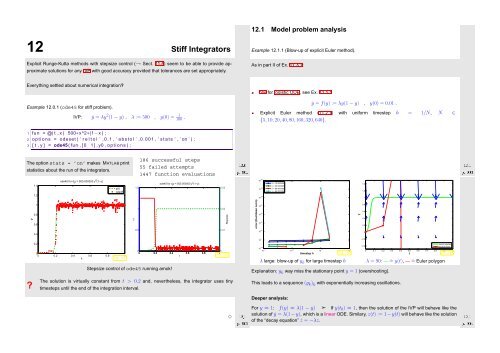
Example 12.0.1 (ode45 for stiff problem).
IVP: ẏ = λy 2 (1 − y) , λ := 500 , y(0) = 1
100 .
IVP for logistic ODE, see Ex. 11.1.1
ẏ = f(y) := λy(1 − y) , y(0) = 0.01 .
Explicit Euler method (11.2.1) with uniform timestep h = 1/N, N ∈
{5, 10, 20, 40, 80, 160, 320, 640}.
1 fun = @( t , x ) 500∗x^2∗(1−x ) ;
2 o p tions = odeset ( ’ r e l t o l ’ , 0 . 1 , ’ a b s t o l ’ ,0.001 , ’ s t a t s ’ , ’ on ’ ) ;
3 [ t , y ] = ode45 ( fun , [ 0 1 ] , y0 , o p tions ) ;
Ôº¼½ ½¾º¼
186 successful steps
The option stats = ’on’ makes MATLAB print
55 failed attempts
statistics about the run of the integrators.
1447 function evaluations
Ôº¼¿ ½¾º½
1.4
1.2
ode45 for d t
y = 500.000000 y 2 (1−y)
y(t)
ode45
1.5
ode45 for d t
y = 500.000000 y 2 (1−y)
0.03
10 120
10 100
10 140 timestep h
λ = 10.000000
λ = 30.000000
λ = 60.000000
λ = 90.000000
1.4
1.2
1
y
?
1
0.8
0.6
0.4
0.2
0
0 0.2 0.4 0.6 0.8 1
t
Fig. 154
Stepsize control of ode45 running amok!
y(t)
1
0.5
0.02
0
0 0.2 0.4 0.6 0.8 1
t
Fig. 155
0 0.2 0.4 0.6 0.8 1 0 0.01
The solution is virtually constant from t > 0.2 and, nevertheless, the integrator uses tiny
timesteps until the end of the integration interval.
Stepsize
error (Euclidean norm)
10 80
10 60
10 40
10 20
10 0
10 −20
10 −3 10 −2 10 −1 10 0
Fig. 156
λ large: blow-up of y k for large timestep h λ = 90: — ˆ= y(t), — ˆ= Euler polygon
Explanation: y k way miss the stationary point y = 1 (overshooting).
This leads to a sequence (y k ) k with exponentially increasing oscillations.
y
0.8
0.6
0.4
0.2
0
−0.2
exact solution
−0.4
explicit Euler
0 0.1 0.2 0.3 0.4 0.6 0.7 0.8 0.5
t
0.9 1
Fig. 157
Ôº¼¾ ½¾º½ ✸
Deeper analysis:
For y ≈ 1: f(y) ≈ λ(1 − y) ➣ If y(t 0 ) ≈ 1, then the solution of the IVP will behave like the
solution of ẏ = λ(1 −y), which is a linear ODE. Similary, z(t) := 1 −y(t) will behave like the solution
of the “decay equation” ż = −λz.
Ôº¼ ½¾º½