Numerical Methods Contents - SAM

0 1 2 3 4 5 6
u(t),v(t)
0.01
0.008
0.006
0.004
0.002
0
−0.002
−0.004
−0.006
−0.008
−0.01
u(t)
v(t)/100
RCL−circuit: R=100.000000, L=1.000000, C=0.000001
time t
Fig. 162
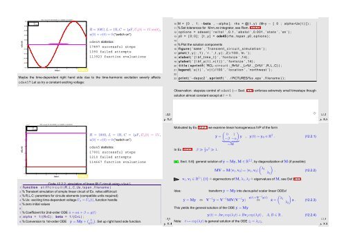
R = 100Ω, L = 1H, C = 1µF, U s (t) = 1V sin(t),
u(0) = v(0) = 0 (“switch on”)
ode45 statistics:
17897 successful steps
1090 failed attempts
113923 function evaluations
Maybe the time-dependent right hand side due to the time-harmonic excitation severly affects
ode45? Let us try a constant exciting voltage:
10 M = [0 , 1 ; −beta , −alpha ] ; rhs = @( t , y ) (M∗y − [ 0 ; alpha∗Us( t ) ] ) ;
11 % Set tolerances for MATLAB integrator, see Rem. 11.5.11
12 o p tions = odeset ( ’ r e l t o l ’ , 0 . 1 , ’ a b s t o l ’ ,0.001 , ’ s t a t s ’ , ’ on ’ ) ;
13 y0 = [ 0 ; 0 ] ; [ t , y ] = ode45 ( rhs , tspan , y0 , o p tions ) ;
14
15 % Plot the solution components
16 figure ( ’name ’ , ’ T r a n sient c i r c u i t s i m u l a t i o n ’ ) ;
17 plot ( t , y ( : , 1 ) , ’ r . ’ , t , y ( : , 2 ) /100 , ’m. ’ ) ;
18 xlabel ( ’ { \ b f time t } ’ , ’ f o n t s i z e ’ ,14) ;
19 ylabel ( ’ { \ b f u ( t ) , v ( t ) } ’ , ’ f o n t s i z e ’ ,14) ;
20 t i t l e ( s p r i n t f ( ’RCL−c i r c u i t : R=%f , L=%f , C=%f ’ ,R, L ,C) ) ;
21 legend ( ’ u ( t ) ’ , ’ v ( t ) /100 ’ , ’ l o c a t i o n ’ , ’ northwest ’ ) ;
22
23 p r i n t ( ’−depsc2 ’ , s p r i n t f ( ’ . . / PICTURES/%s . eps ’ , filename ) ) ;
Observation: stepsize control of ode45 (→ Sect. 11.5) enforces extremely small timesteps though
solution almost constant except at t = 0.
Ôº½¿ ½¾º¾
Ôº½ ½¾º¾ ✸
u(t),v(t)
RCL−circuit: R=100.000000, L=1.000000, C=0.000001
2 x 10−3 u(t)
v(t)/100
0
−2
−4
−6
−8
−10
−12
0 1 2 3 4 5 6
time t
Fig. 163
R = 100Ω, L = 1H, C = 1µF, U s (t) = 1V,
u(0) = v(0) = 0 (“switch on”)
ode45 statistics:
17901 successful steps
1210 failed attempts
114667 function evaluations
Code 12.2.2: simulation of linear RLC circuit using ode45
1 function s t i f f c i r c u i t (R, L ,C, Us , tspan , filename )
2 % Transient simulation of simple linear circuit of Ex. refex:stiffcircuit
3 % R,L,C: paramters for circuits elements (compatible units required)
4 % Us: exciting time-dependent voltage U s = U s (t), function handle
5 % zero initial values
6
7 % Coefficient for 2nd-order ODE ü + α ˙u + β = g(t)
8 alpha = 1 / (R∗C) ; beta = 1 / (C∗L ) ;
9 % Conversion to 1st-order ODE y = My + ( 0
g(t))
. Set up right hand side function.
Ôº½ ½¾º¾
Motivated by Ex. 12.2.1 we examine linear homogeneous IVP of the form
( )
0 1
ẏ = y , y(0) = y
−β −α
0 ∈ R 2 . (12.2.1)
} {{ }
=:M
In Ex .12.2.1: β ≫ 1 4 α2 ≫ 1.
[40, Sect. 5.6]: general solution of ẏ = My, M ∈ R 2,2 , by diagonalization of M (if possible):
( )
λ1
MV = M (v 1 ,v 2 ) = (v 1 ,v 2 ) . (12.2.2)
λ2
Idea:
v 1 ,v 2 ∈ R 2 \ {0} ˆ= eigenvectors of M, λ 1 ,λ 2 ˆ= eigenvalues of M, see Def. 5.1.1.
transform ẏ = My into decoupled scalar linear ODEs!
ẏ = My ⇔ V −1 ẏ = V −1 MV(V −1 y)
This yields the general solution of the ODE ẏ = My
z(t):=V −1 y(t)
⇔ ż =
(
λ1
λ2
)
z . (12.2.3)
Ôº½ ½¾º¾
Note: t ↦→ exp(λ i t) is general solution of the ODE ż i = λ i z i .
y(t) = Av 1 exp(λ 1 t) + Bv 2 exp(λ 2 t) , A,B ∈ R . (12.2.4)